この章の地図Map of this note

• 1同種粒子の交換対称性Exchange symmetry of identical particles
• 2ボース分布とフェルミ分布Bose and Fermi distributions
• 3状態密度と三次元理想気体Density of states & the 3D gas
• 4高温からの展開Expansion from high temperature
• 5低温のボース気体（BEC）The cold Bose gas (BEC)
• 6低温のフェルミ気体The cold Fermi gas
• 7物理数学のまとめMathematical appendix

全体を通して、\(g\) は一粒子状態の内部縮重度（同じ運動状態に乗る内部状態の数）を表します。外場がなく、すべてのスピン状態を統計に含める場合は \(g=2s+1\)——主な例はスピン \(s=\dfrac12\) の \(g=2\) です。スピン \(0\) のボース粒子（液体 \(^4\mathrm{He}\)）や、単一の内部状態に偏極させた冷却原子気体のような一成分気体では \(g=1\) とします。温度依存の熱力学量は、§3.5 の図 1 に数値計算の結果としてまとめてあります。

Throughout, \(g\) denotes the internal degeneracy of a single-particle state (how many internal states ride on each orbital state). With no external field and all spin states included, \(g=2s+1\) — the main example being spin \(s=\dfrac12\) with \(g=2\). For spin-\(0\) bosons (liquid \(^4\mathrm{He}\)) and for one-component gases such as cold atoms polarised into a single internal state, \(g=1\). The temperature dependence of the thermodynamic quantities is collected, from the numerics, in Fig. 1 of §3.5.

1同種粒子の交換対称性 —— すべてはここからExchange symmetry of identical particles — where everything begins

古典力学では、同じ種類の粒子が二つあっても、それぞれを「追跡」できます。時刻ゼロにどこにいたかを覚えておけば、軌道をたどって「1番の粒子」「2番の粒子」と言い続けられるからです。量子力学ではこれが原理的に不可能になります。粒子は波動関数として広がり、二つの波束が一度重なってから離れると、「どちらがどちらだったか」を知る手段はもう存在しません。同種粒子は区別できない——量子統計の物語は、この一点から始まります。

In classical mechanics you can always keep track of two particles of the same kind: remember where each one was at time zero and follow its trajectory, and you may keep calling them "particle 1" and "particle 2". Quantum mechanics makes this impossible in principle. Particles are spread-out wavefunctions, and once two wave packets overlap and separate again, there is no way left to tell which was which. Identical particles are indistinguishable — and the whole story of quantum statistics grows out of this single fact.

1.1　入れ替えの演算子と符号 \(\sigma\)1.1　The exchange operator and the sign \(\sigma\)

区別できない以上、粒子の「ラベル」の付け替えで物理が変わってはいけません。二粒子の波動関数を \(\Psi(x_1,x_2)\) と書きます（\(x\) は位置とスピンをまとめた記号です）。ラベルを入れ替える交換演算子 \(\hat P\) を

If the particles cannot be distinguished, relabelling them must not change the physics. Write the two-particle wavefunction as \(\Psi(x_1,x_2)\), where \(x\) stands for position and spin together. Define the exchange operator \(\hat P\) by

で定義しましょう。二回入れ替えれば完全に元に戻るので \(\hat P^2=1\)。したがって \(\hat P\) の固有値 \(\sigma\) は

Swapping twice restores the original completely, so \(\hat P^2=1\). The eigenvalues \(\sigma\) of \(\hat P\) therefore obey

の二つしかありません。さらに、同種粒子系のハミルトニアンはラベルの付け替えで不変（\([\hat P,\hat H]=0\)）なので、この符号は時間が経っても変わりません。つまり、このノートで扱う通常の三次元の同種多粒子系は、入れ替えても波動関数が変わらない \(\sigma=+1\)（対称）の世界か、符号だけ反転する \(\sigma=-1\)（反対称）の世界か、どちらかに恒久的に属します。

— only two possibilities. Moreover, the Hamiltonian of identical particles is invariant under relabelling (\([\hat P,\hat H]=0\)), so this sign never changes in time. Every ordinary three-dimensional system of identical particles — the setting of this note — thus belongs permanently to one of two worlds: the \(\sigma=+1\) world, where the wavefunction is symmetric under exchange, or the \(\sigma=-1\) world, where it is antisymmetric.

1.2　どちらの世界か：スピン統計定理1.2　Which world? The spin–statistics theorem

どちらの世界に属するかを決めているのが、粒子のスピンです。相対論的な場の量子論から、整数スピンの粒子は \(\sigma=+1\)、半整数スピンの粒子は \(\sigma=-1\) であることが示せます（スピン統計定理）。\(\sigma=+1\) の粒子をボース粒子、\(\sigma=-1\) の粒子をフェルミ粒子と呼びます。光子（スピン \(1\)）はボース粒子、電子（スピン \(\dfrac12\)）はフェルミ粒子です。複合粒子では、中に含まれるフェルミ粒子の数が偶数ならボース粒子、奇数ならフェルミ粒子になります：\(^4\mathrm{He}\) 原子（陽子2＋中性子2＋電子2 ＝ 偶数）はボース粒子、\(^3\mathrm{He}\) 原子（中性子が一つ減って奇数）はフェルミ粒子です。同じヘリウムなのに低温での振る舞いが劇的に違う——その理由は、この符号一つに遡ります。

What decides the world is the particle's spin. Relativistic quantum field theory shows that integer-spin particles have \(\sigma=+1\) and half-integer-spin particles have \(\sigma=-1\) (the spin–statistics theorem). Particles with \(\sigma=+1\) are called bosons, those with \(\sigma=-1\) fermions. The photon (spin \(1\)) is a boson; the electron (spin \(\dfrac12\)) is a fermion. For composite particles, an even number of constituent fermions makes a boson and an odd number makes a fermion: a \(^4\mathrm{He}\) atom (2 protons + 2 neutrons + 2 electrons = even) is a boson, while \(^3\mathrm{He}\) (one neutron fewer, odd) is a fermion. Same element, dramatically different low-temperature behaviour — all traceable to this single sign.

1.3　二粒子で見る帰結：パウリの排他原理1.3　The consequence, seen with two particles: the Pauli principle

符号 \(\sigma\) の威力は、粒子二つで既にはっきり現れます。互いに直交する規格化された一粒子状態 \(\psi_a\) と \(\psi_b\) に粒子を一つずつ入れた二粒子状態は、対称性の要請を満たすように

The power of the sign \(\sigma\) already shows with just two particles. Putting one particle in each of two mutually orthogonal, normalised single-particle states \(\psi_a\) and \(\psi_b\), the two-particle state that respects the symmetry requirement is

と書けます（\(\hat P\Psi_\sigma=\sigma\Psi_\sigma\) を確かめてみてください）。ここで二つの粒子を同じ状態に入れてみます（\(b=a\)）。このとき「\(\psi_a\) と \(\psi_b\) が直交する」という前提は崩れるので、規格化因子 \(\dfrac{1}{\sqrt2}\) はそのままでは使えません。そこで規格化はいったん脇に置き、（反）対称化した組み合わせの形だけを見ます。\(\sigma=+1\) なら \(\Psi_+\propto\psi_a(x_1)\psi_a(x_2)\)——形は立派に生き残るので、あらためて規格化し直せば済みます。ところが \(\sigma=-1\) では

(check that \(\hat P\Psi_\sigma=\sigma\Psi_\sigma\)). Now try to put both particles in the same state, \(b=a\). The premise that \(\psi_a\) and \(\psi_b\) are orthogonal now fails, so the factor \(\dfrac{1}{\sqrt2}\) no longer normalises anything — set normalisation aside, then, and look only at the shape of the (anti)symmetrised combination. For \(\sigma=+1\), \(\Psi_+\propto\psi_a(x_1)\psi_a(x_2)\): the shape survives, and one simply renormalises. But for \(\sigma=-1\),

規格化でどう直そうにも、状態そのものが恒等的に零です。フェルミ粒子は、同じ一粒子状態に二つ入ることができない——これがパウリの排他原理です。何かの力が押し返しているのではなく、反対称性からの純粋に数学的な帰結である点に注意してください。

the combination is identically zero — no normalisation can rescue a state that is not there. Two fermions cannot occupy the same single-particle state — this is the Pauli exclusion principle. Note that no force is pushing them apart: it is a purely mathematical consequence of antisymmetry.

1.4　「誰がどこ」から「どこに何個」へ1.4　From "who is where" to "how many in each state"

区別できない粒子の多体状態を指定するのに、「どの粒子がどの状態にいるか」を語る必要はもうありません。ラベルに意味がないのだから、意味を持つ情報は「各一粒子状態 \(q\) に何個の粒子が入っているか」——占有数の組 \(\{n_q\}\)——だけです。相互作用のない系のエネルギー固有状態——フォック基底の各基底状態——は \(|n_{q_1},n_{q_2},n_{q_3},\cdots\rangle\) というケットで指定できます（一般の量子状態は、これらの重ね合わせです）。そして、いま見た通り、許される \(n_q\) の値が二つの世界で違います。この「数の言葉」への乗り換えが、次節からの統計力学を驚くほど簡単にしてくれます。

To specify a many-body state of indistinguishable particles we no longer need to say "which particle is in which state". Since the labels mean nothing, the only meaningful information is how many particles occupy each single-particle state \(q\) — the set of occupation numbers \(\{n_q\}\). Each basis state of the Fock basis — each energy eigenstate of the non-interacting system — is specified by the ket \(|n_{q_1},n_{q_2},n_{q_3},\cdots\rangle\) (a general quantum state is a superposition of these), and as we have just seen, the allowed values of \(n_q\) differ between the two worlds. This switch to counting language is what makes the statistical mechanics of the coming sections astonishingly simple.

コラム：ボース粒子でもフェルミ粒子でもない粒子はいないのか？Column: is there a particle that is neither boson nor fermion?クリックで展開click to expand

1.1 で定義した \(\hat P\) は、波動関数の粒子ラベルを入れ替える演算子でした。これは空間次元によらず、定義から \(\hat P^2=1\) を満たします。二次元で事情が変わるのは、粒子を空間の中で実際に動かして交換する操作のほうです。ラベル交換と区別して、これを \(\hat B\) と書きましょう。粒子を二回交換することは、片方の粒子がもう片方の周りをぐるりと一周することと同じです（一回目で入れ替わり、二回目で元に戻る——軌跡をつなげると一つの閉じた輪になります）。「二回交換＝何もしない」と言えるのは、この輪を、相手にぶつからずに一点まで縮められるときだけ。交換が波動関数に位相だけを与えるなら \(\hat B\Psi=e^{i\theta}\Psi\) と書けます——この \(\theta\) が何に縛られるかを、次の絵で見ましょう。

The operator \(\hat P\) of 1.1 swaps the labels in the wavefunction; by its very definition it satisfies \(\hat P^2=1\) in any dimension. What changes in two dimensions is the physical operation of moving the particles around each other to exchange them — call it \(\hat B\), to keep it distinct from the label swap. Exchanging twice equals one particle making a full loop around the other (swap once, swap back — the joined trajectory is one closed loop), and "double exchange = doing nothing" holds only when that loop can be shrunk to a point without ever touching the other particle. If the exchange merely multiplies the wavefunction by a phase, we may write \(\hat B\Psi=e^{i\theta}\Psi\) — and the picture below decides what constrains this \(\theta\).

「二回交換」＝「B が A の周りを一周」で、輪は B の軌跡です。三次元では輪を面の外へ持ち上げ、A を避けて一点まで縮められる——二回交換は「何もしない」と連続的につながり、\(\sigma^2=1\)。縮めている間、輪がどこにあるかは重要ではなく、A に触れないことだけが要です。二次元では輪が平面に閉じ込められ、A を囲んだまま外せません。

"Double exchange" = "B loops once around A"; the loop is the trajectory of B. In 3D the loop can be lifted off the plane and shrunk to a point while avoiding A — double exchange connects continuously to "doing nothing", so \(\sigma^2=1\). Where the loop sits while it shrinks is irrelevant; all that matters is never touching A. In 2D the loop is trapped in the plane and can never stop encircling A.

机の上のコマの周りに紐を一周張ることを想像してください。紐が机から離れられないなら、コマを避けて紐を回収することはできません。でも三次元なら、紐を持ち上げて頭の上を通せばするりと外せます。この「持ち上げる」という迂回路が、三次元にはあって二次元にはない——それだけの違いが、統計性の運命を分けます。

Picture a string looped around a game piece on a table. If the string must stay on the table, you cannot retrieve it without hitting the piece. In three dimensions you simply lift the string over the top and it slips free. That "lift" — a detour that exists in 3D but not in 2D — is the entire difference, and it decides the fate of statistics.

三次元では二回交換が「何もしない」と連続変形でつながるので、交換の位相 \(e^{i\theta}\) は \(e^{2i\theta}=1\) を満たすしかなく、\(\sigma=\pm1\)——ボース統計とフェルミ統計だけが許されます。二次元ではその制約が消え、任意の位相 \(e^{i\theta}\) が許されます。any（任意の）phase を持てる粒子、という意味でエニオン（anyon）と呼ばれます。数学的には、三次元の交換が「置換群」で記述されるのに対し、二次元の交換は紐の絡み方まで区別する「組みひも群」で記述される、と言い換えられます。これは絵空事ではなく、強磁場中の二次元電子系（分数量子ホール効果）の準粒子はエニオンであると予言され、2020年前後の干渉実験で、分数量子ホール系の（アーベル型）準粒子について統計位相が直接確認されました。この先で組み立てていく量子統計は「\(\pm1\) の世界」の物理です。次元を一つ落とすだけで統計性そのものが連続パラメータになる——統計性はトポロジーの産物なのです。

In 3D, double exchange deforms continuously into "doing nothing", so the exchange phase \(e^{i\theta}\) must satisfy \(e^{2i\theta}=1\): only \(\sigma=\pm1\), Bose or Fermi. In 2D that constraint evaporates and any phase \(e^{i\theta}\) is allowed — hence anyons. Mathematically, 3D exchanges form the permutation group, while 2D exchanges form the braid group, which remembers how strands wind. And this is not science fiction: quasiparticles of the fractional quantum Hall effect were predicted to be anyons, and interference experiments around 2020 confirmed the statistical phase directly for (abelian) fractional-quantum-Hall quasiparticles. The quantum statistics we build from here on is the physics of the "\(\pm1\) world"; drop one dimension and statistics itself becomes a continuous parameter — statistics is a child of topology.

2ボース分布とフェルミ分布Bose and Fermi distributions

相互作用のない同種粒子系では、全エネルギーと全粒子数が、一粒子固有エネルギー \(\varepsilon_q\) とその占有数 \(n_q\) だけで書けます。ここで \(q\) は一粒子状態を指定する量子数の組です。

For a system of identical, non-interacting particles the total energy and total particle number are fixed entirely by the single-particle eigen-energies \(\varepsilon_q\) and their occupation numbers \(n_q\), where \(q\) labels a single-particle state.

第1節で見たように、多粒子状態 \(\nu\) は占有数の組 \(\{n_q\}\) で完全に決まり、しかも \(n_q\) の取れる値は交換対称性が既に決めてくれています。スピン統計定理により、粒子のスピン \(s\) が整数か半整数かに応じて、

As §1 showed, a many-body state \(\nu\) is completely specified by the occupations \(\{n_q\}\), and the allowed values of \(n_q\) have already been fixed by exchange symmetry. By the spin–statistics theorem, depending on whether the spin \(s\) is integer or half-integer,

以下ではこの符号 \(\sigma=\pm1\)——第1節の交換の符号そのもの——を使って、両統計を一括で扱います。ボース粒子は同じ状態に何個でも入れるのに対し、フェルミ粒子はパウリ原理で高々一個。この一行の違いが、以下すべての物理を生みます。

The sign \(\sigma=\pm1\) — the very exchange sign of §1 — lets us treat both cases at once. Bosons can pile arbitrarily many particles into one state; fermions, by the Pauli principle, admit at most one. Everything below flows from this single line.

なぜ大正準集団かWhy the grand canonical ensemble

占有数の和 \(N_\nu=\sum_q n_q\) を一定に固定すると、状態和が数学的に厄介になります。そこで粒子数を固定せず、化学ポテンシャル \(\mu\) を通じて平均的にだけ制御する大正準集団を使います。これは単なる技術的都合で、本文で扱う巨視的な平均熱力学量については、熱力学極限で集団の選び方によらず同じ結果になります。大分配関数は

Fixing the total occupation \(N_\nu=\sum_q n_q\) makes the sum over states awkward. So instead of fixing the particle number we control it only on average, through a chemical potential \(\mu\): the grand canonical ensemble. This is a technical convenience — for the macroscopic average quantities treated in this note, the choice of ensemble gives the same results in the thermodynamic limit. The grand partition function is

肝は三段目、「多粒子状態 \(\{n_q\}\) 全体にわたる和」を「各 \(n_q\) についての和の積」に分解するところです。二段構えで見ると分かりやすい。まず、指数関数の肩は占有数の和なので、指数法則 \(e^{a+b}=e^{a}e^{b}\) によって状態ごとの因子の積にほどけます：

The crux is the third step, where the sum over all many-body configurations \(\{n_q\}\) is turned into a product of independent sums over each \(n_q\). It is clearest in two stages. First, the exponent is a sum over occupations, so by \(e^{a+b}=e^{a}e^{b}\) the exponential unravels into a product of one factor per state:

次に、\(\{n_q\}\) についての和とは「\(n_{q_1}\) の許される値、\(n_{q_2}\) の許される値、……をそれぞれ独立に走らせる多重和」のことです。各因子は自分の \(n_q\) にしか依存しないので、多重和は因子ごとの和の積に分かれます。信じられないときは、いちばん小さな例で確かめるのが一番です。一粒子状態が二つしかないフェルミ粒子系（\(n_1,n_2\in\{0,1\}\)）で、\(a\equiv e^{-\beta(\varepsilon_1-\mu)}\)、\(b\equiv e^{-\beta(\varepsilon_2-\mu)}\) と略記すると、多粒子状態は \(|0,0\rangle,|1,0\rangle,|0,1\rangle,|1,1\rangle\) の4つで、

Second, the sum over \(\{n_q\}\) means a multiple sum in which \(n_{q_1}\), \(n_{q_2}\), … each run independently over their allowed values. Since each factor depends only on its own \(n_q\), the multiple sum splits into a product of single sums. When in doubt, check the smallest example: a Fermi system with just two single-particle states (\(n_1,n_2\in\{0,1\}\)). Writing \(a\equiv e^{-\beta(\varepsilon_1-\mu)}\), \(b\equiv e^{-\beta(\varepsilon_2-\mu)}\), the many-body states are \(|0,0\rangle,|1,0\rangle,|0,1\rangle,|1,1\rangle\), and

右辺の積を展開すると、4つの多粒子状態の寄与が過不足なく一つずつ現れる——これが「和の積への分解」の中身です。状態数が増えても、ボース粒子のように \(n_q\) が無限に走っても、同じ理屈がそのまま通ります。あとは各因子を実行するだけです。ボース粒子では等比級数 \(1+y+y^2+\cdots=\dfrac{1}{1-y}\)（\(y=e^{-\beta(\varepsilon_q-\mu)}\lt1\)）、フェルミ粒子では \(n_q=0,1\) の二項和 \(1+y\)。両者は \([\,1-\sigma e^{-\beta(\varepsilon_q-\mu)}\,]^{-\sigma}\) という一つの式にまとまります。

Expanding the product on the right reproduces the four many-body contributions exactly once each — that is all the "factorisation into a product of sums" means. The same logic survives any number of states, and even the infinite range of \(n_q\) for bosons. It only remains to evaluate each factor: a geometric series \(1+y+y^2+\cdots=\dfrac{1}{1-y}\) for bosons (\(y=e^{-\beta(\varepsilon_q-\mu)}\lt1\)), and the two-term sum \(1+y\) for fermions. Both collapse into the single expression \([\,1-\sigma e^{-\beta(\varepsilon_q-\mu)}\,]^{-\sigma}\).

グランドポテンシャル \(\Omega=-k_{\mathrm B}T\ln\mathcal{Z}_G\) は、対数が積を和に変える（\(\ln\prod_q=\sum_q\ln\)、冪 \(-\sigma\) は係数として前に出る）ことから、

The grand potential \(\Omega=-k_{\mathrm B}T\ln\mathcal{Z}_G\) follows because the logarithm turns the product into a sum (\(\ln\prod_q=\sum_q\ln\), the power \(-\sigma\) coming out as a coefficient):

この形は、体積 \(V\) が独立変数として適切でない場合（例えば調和振動子ポテンシャルに捕捉された冷却原子気体）にもそのまま使えるのが利点です。

A virtue of this form is that it still works when the volume \(V\) is not a natural variable — for instance, cold atoms held in a harmonic trap.

平均占有数：ボース分布とフェルミ分布Mean occupation: the Bose and Fermi distributions

平均粒子数は、\(d\Omega=-S\,dT-P\,dV-N\,d\mu\) から \(N=-\left(\dfrac{\partial\Omega}{\partial\mu}\right)_{\!T,V}\) で得られます。微分を実行しましょう。対数の微分から分布関数が現れます：

The mean particle number follows from \(d\Omega=-S\,dT-P\,dV-N\,d\mu\) as \(N=-\left(\dfrac{\partial\Omega}{\partial\mu}\right)_{\!T,V}\). Let us carry out the derivative — the distribution function emerges from differentiating the logarithm:

途中で \(\sigma^2=1\)、最後に分子・分母へ \(e^{\beta(\varepsilon_q-\mu)}\) を掛けました。和の各項が「状態 \(q\) を占める平均粒子数」\(\bar n_q\) です。内部エネルギーは平均の線形性から \(U=\langle E_\nu\rangle=\bigl\langle\sum_q\varepsilon_q n_q\bigr\rangle=\sum_q\varepsilon_q\langle n_q\rangle\) となり、同じ \(\bar n_q\) で書けます。まとめて：

(we used \(\sigma^2=1\), then multiplied numerator and denominator by \(e^{\beta(\varepsilon_q-\mu)}\)). Each term of the sum is the mean number of particles occupying state \(q\), \(\bar n_q\). The internal energy follows from linearity of the average, \(U=\langle E_\nu\rangle=\bigl\langle\sum_q\varepsilon_q n_q\bigr\rangle=\sum_q\varepsilon_q\langle n_q\rangle\), with the same \(\bar n_q\). Collecting:

\(\sigma=+1\) がボース分布、\(\sigma=-1\) がフェルミ分布です。フェルミ分布は \(0\le\bar n_q\le1\) に収まりますが、ボース分布は \(\varepsilon_q\to\mu\) で発散し得ます（これが後の BEC の芽です）。\(e^{\beta(\varepsilon_q-\mu)}\gg1\) の高温・希薄極限では、両者とも次のマクスウェル–ボルツマン分布に帰着します。

\(\sigma=+1\) is the Bose distribution, \(\sigma=-1\) the Fermi distribution. The Fermi distribution stays within \(0\le\bar n_q\le1\), while the Bose distribution can diverge as \(\varepsilon_q\to\mu\) — the seed of the condensation to come. In the hot, dilute limit \(e^{\beta(\varepsilon_q-\mu)}\gg1\) both reduce to the Maxwell–Boltzmann distribution:

方程式 \(N=\sum_q\bar n_q\) は、逆に「\(N\) を与えて \(\mu=\mu(T,N)\) を決める式」とも読めます。この関係で独立変数を \(\mu\) から \(N\)（平均粒子数）へ移すのが、以下の計算の常道です。

Read backwards, \(N=\sum_q\bar n_q\) is the equation that determines \(\mu=\mu(T,N)\) for a given \(N\). Trading the independent variable \(\mu\) for \(N\) (the mean particle number) this way is the standard move in what follows.

コラム：ボース分布とフェルミ分布は一瞬で導けるColumn: the Bose and Fermi distributions in one breathクリックで展開click to expand

実は \(\bar n_q\) は、\(\Omega\) を経由しなくても一つの準位に注目するだけで導けます。根拠は上の因数分解そのものです。\(\mathcal{Z}_G\) が準位ごとの因子の積に分かれたということは、各準位の占有数は互いに統計的に独立で、準位 \(q\) だけを見れば「占有数 \(n\) が重み \(e^{-\beta(\varepsilon_q-\mu)n}\) で分布する」ミニ大正準集団になっている、ということです。だから期待値は

In fact \(\bar n_q\) can be derived by looking at a single level, with no detour through \(\Omega\). The justification is the factorisation above: since \(\mathcal{Z}_G\) splits into one factor per level, the occupations of different levels are statistically independent, and level \(q\) on its own is a mini grand-canonical ensemble in which the occupation \(n\) carries the weight \(e^{-\beta(\varepsilon_q-\mu)n}\). Hence

\[ \bar n_q=\langle n_q\rangle =\frac{\displaystyle\sum_{n} n\,e^{-\beta(\varepsilon_q-\mu)n}}{\displaystyle\sum_{n} e^{-\beta(\varepsilon_q-\mu)n}}, \]

和は許される \(n\) だけを走ります。フェルミ粒子がいちばん速い：\(n=0,1\) しかないので、\(y\equiv e^{-\beta(\varepsilon_q-\mu)}\) と略記して

where \(n\) runs over the allowed values only. Fermions are fastest: with just \(n=0,1\), and writing \(y\equiv e^{-\beta(\varepsilon_q-\mu)}\),

\[ \bar n_q=\frac{0\cdot1+1\cdot y}{1+y}=\frac{y}{1+y}=\frac{1}{e^{\beta(\varepsilon_q-\mu)}+1}. \]

ボース粒子は \(n=0,1,2,\dots\) の等比級数が二本出るだけです。\(\sum_{n=0}^{\infty}y^{n}=\dfrac{1}{1-y}\) と、それを微分して得られる \(\sum_{n=0}^{\infty}n\,y^{n}=\dfrac{y}{(1-y)^{2}}\) を使えば、

For bosons we just need two geometric series over \(n=0,1,2,\dots\): \(\sum_{n=0}^{\infty}y^{n}=\dfrac{1}{1-y}\) and its derivative \(\sum_{n=0}^{\infty}n\,y^{n}=\dfrac{y}{(1-y)^{2}}\). Then

\[ \bar n_q=\frac{0\cdot1+1\cdot y+2\,y^{2}+\cdots}{1+y+y^{2}+\cdots} =\frac{y/(1-y)^{2}}{1/(1-y)}=\frac{y}{1-y} =\frac{1}{e^{\beta(\varepsilon_q-\mu)}-1}. \]

どちらも本文の式 \(\eqref{eq:nbar}\) と一致します。分布の形を忘れたら、この最短ルートで30秒で再導出できます——準位ごとの独立性がすべてを支えている、という見方ごと覚えておくのがおすすめです。

Both agree with \(\eqref{eq:nbar}\) of the main text. Forget the distributions, and this shortest route re-derives them in thirty seconds — powered entirely by the level-by-level independence.

エントロピーと熱容量Entropy and heat capacity

グランドポテンシャルの全微分は \(d\Omega=-S\,dT-P\,dV-N\,d\mu\) なので、エントロピーは \(S=-\left(\dfrac{\partial\Omega}{\partial T}\right)_{\!V,\mu}\) で得られます。\(T\) 微分は \(\beta=\dfrac{1}{k_{\mathrm B}T}\) の微分に直すのが便利です：\(\dfrac{d\beta}{dT}=-\dfrac{1}{k_{\mathrm B}T^{2}}=-k_{\mathrm B}\beta^{2}\) より

The total differential of the grand potential is \(d\Omega=-S\,dT-P\,dV-N\,d\mu\), so the entropy is \(S=-\left(\dfrac{\partial\Omega}{\partial T}\right)_{\!V,\mu}\). It is convenient to trade the \(T\)-derivative for a \(\beta\)-derivative, \(\beta=\dfrac{1}{k_{\mathrm B}T}\): since \(\dfrac{d\beta}{dT}=-\dfrac{1}{k_{\mathrm B}T^{2}}=-k_{\mathrm B}\beta^{2}\),

ここに \(\Omega=\dfrac{\sigma}{\beta}\sum_q\ln\bigl[1-\sigma e^{-\beta(\varepsilon_q-\mu)}\bigr]\) を入れ、積の微分で二項に分けます。第二項に現れる微分は

Insert \(\Omega=\dfrac{\sigma}{\beta}\sum_q\ln\bigl[1-\sigma e^{-\beta(\varepsilon_q-\mu)}\bigr]\) and apply the product rule. The derivative appearing in the second term is

ここで分子・分母に \(e^{\beta(\varepsilon_q-\mu)}\) を掛けると \(\dfrac{e^{-\beta(\varepsilon_q-\mu)}}{1-\sigma e^{-\beta(\varepsilon_q-\mu)}}=\dfrac{1}{e^{\beta(\varepsilon_q-\mu)}-\sigma}=\bar n_q\) となることを使いました。まとめると（\(\sigma^2=1\) に注意）、

where multiplying numerator and denominator by \(e^{\beta(\varepsilon_q-\mu)}\) gives \(\dfrac{e^{-\beta(\varepsilon_q-\mu)}}{1-\sigma e^{-\beta(\varepsilon_q-\mu)}}=\dfrac{1}{e^{\beta(\varepsilon_q-\mu)}-\sigma}=\bar n_q\). Collecting the two terms (note \(\sigma^2=1\)),

これを占有数 \(\bar n_q\) だけで書き直します。鍵は、分布関数の定義 \(\bar n_q=\dfrac{1}{e^{\beta(\varepsilon_q-\mu)}-\sigma}\) を「逆に解いた」次の二つの恒等式です：

Now rewrite everything in terms of \(\bar n_q\) alone. The key is the following pair of identities, obtained by solving the definition \(\bar n_q=\dfrac{1}{e^{\beta(\varepsilon_q-\mu)}-\sigma}\) backwards:

二つを代入して整理すると、一状態あたりの寄与は

Substituting both and collecting, the contribution of one state becomes

そして \(\sigma+\bar n_q=\sigma(1+\sigma\bar n_q)\)（\(\sigma^2=1\)）を使えば、最終形に到達します。

and using \(\sigma+\bar n_q=\sigma(1+\sigma\bar n_q)\) (again \(\sigma^2=1\)) we reach the final form:

フェルミ統計（\(\sigma=-1\)）ではこれは \(-k_{\mathrm B}\sum_q[\bar n_q\ln\bar n_q+(1-\bar n_q)\ln(1-\bar n_q)]\) となります。「状態 \(q\) が占有されている確率 \(\bar n_q\)、空である確率 \(1-\bar n_q\)」の二値エントロピーの和——という、これ以上ないほど直感的な形です。

For Fermi statistics (\(\sigma=-1\)) this is \(-k_{\mathrm B}\sum_q[\bar n_q\ln\bar n_q+(1-\bar n_q)\ln(1-\bar n_q)]\): a sum of binary entropies, "state \(q\) occupied with probability \(\bar n_q\), empty with probability \(1-\bar n_q\)" — as intuitive as it gets.

熱容量Heat capacity

熱容量は \(C=T\left(\dfrac{\partial S}{\partial T}\right)_{\!N}\) で定義されますが、体積と粒子数を固定すると \(dU=T\,dS\) なので、これは \(C=\left(\dfrac{\partial U}{\partial T}\right)_{\!N}\) と同じことです。後者の方が計算しやすいので、\(U=\sum_q\varepsilon_q\bar n_q\) を温度で微分します。占有数は \(x\equiv\beta(\varepsilon_q-\mu)=\dfrac{\varepsilon_q-\mu(T)}{k_{\mathrm B}T}\) を通して温度に依存するので、連鎖律で

The heat capacity is defined as \(C=T\left(\dfrac{\partial S}{\partial T}\right)_{\!N}\); but at fixed volume and particle number \(dU=T\,dS\), so this equals \(C=\left(\dfrac{\partial U}{\partial T}\right)_{\!N}\), which is easier to compute. Differentiate \(U=\sum_q\varepsilon_q\bar n_q\) in \(T\). The occupation depends on temperature through \(x\equiv\beta(\varepsilon_q-\mu)=\dfrac{\varepsilon_q-\mu(T)}{k_{\mathrm B}T}\), so by the chain rule

\(x\) の温度微分では、分母の \(T\) と、粒子数を保つために動く \(\mu(T)\) の両方が効きます：

In \(\dfrac{\partial x}{\partial T}\), both the explicit \(T\) in the denominator and the drift of \(\mu(T)\) (needed to conserve particle number) contribute:

ここで粒子数一定の条件 \(\sum_q\dfrac{\partial\bar n_q}{\partial T}=\dfrac{dN}{dT}=0\) に注目します。ここでの温度微分は、\(N\) を一定に保つよう \(\mu(T)\) が動くぶんまで込めた全微分です——そもそも \(\dfrac{\partial\mu}{\partial T}\) の値は、条件 \(0=\left(\dfrac{\partial N}{\partial T}\right)_{\!\mu}+\left(\dfrac{\partial N}{\partial\mu}\right)_{\!T}\dfrac{\partial\mu}{\partial T}\) から決まります。この零を使うと、\(C=\sum_q\varepsilon_q\,\dfrac{\partial\bar n_q}{\partial T}\) から \(\mu\sum_q\dfrac{\partial\bar n_q}{\partial T}=0\) を自由に引けるので、\(\varepsilon_q\) を \(\varepsilon_q-\mu=k_{\mathrm B}T\,x\) に置き換えられます：

Now use particle-number conservation, \(\sum_q\dfrac{\partial\bar n_q}{\partial T}=\dfrac{dN}{dT}=0\) — a total derivative, including the drift of \(\mu(T)\) that keeps \(N\) fixed; indeed \(\dfrac{\partial\mu}{\partial T}\) is determined precisely by \(0=\left(\dfrac{\partial N}{\partial T}\right)_{\!\mu}+\left(\dfrac{\partial N}{\partial\mu}\right)_{\!T}\dfrac{\partial\mu}{\partial T}\). Since we may freely subtract \(\mu\sum_q\dfrac{\partial\bar n_q}{\partial T}=0\) from \(C=\sum_q\varepsilon_q\,\dfrac{\partial\bar n_q}{\partial T}\), we can replace \(\varepsilon_q\) by \(\varepsilon_q-\mu=k_{\mathrm B}T\,x\):

\(\dfrac{\partial\mu}{\partial T}\) の項は、粒子数を一定に保つために化学ポテンシャルが温度とともに動くことの反映です。フェルミ気体と、ボース気体の正常相では、この項を忘れてはいけません。一方、理想ボース気体の凝縮相では熱力学極限で \(\mu=0\) に固定されるため、この項は消え、かわりに 5.2 のように凝縮粒子数を別に扱います。

The \(\dfrac{\partial\mu}{\partial T}\) term reflects the drift of the chemical potential required to hold the particle number fixed. It must be kept for the Fermi gas and for the normal phase of the Bose gas; in the condensed phase of the ideal Bose gas, where \(\mu=0\) is pinned in the thermodynamic limit, it drops out and the condensate number is booked separately instead (5.2).

コラム：1926年——フェルミとディラック、そして「教皇」Column: 1926 — Fermi, Dirac, and "the Pope"クリックで展開click to expand

E. Fermi

1901–1954

P. A. M. Dirac

1902–1984

フェルミ分布は 1926 年、フェルミとディラックによって相次いで独立に発見されました。まず2月、ローマの24歳のフェルミが、パウリの排他原理（1.3）を理想気体に課すと何が起きるかを計算しました。数か月後、ケンブリッジのディラックが、波動関数の反対称性（\(\sigma=-1\)）から同じ分布を導きます。自分の先行に気づいたフェルミは丁寧な手紙をディラックに送り、ディラックは以後これを「フェルミ統計」と呼びました。のちに \(\sigma=-1\) の粒子を fermion、\(\sigma=+1\) の粒子を boson と命名したのもディラックです。

The Fermi distribution was discovered independently, in quick succession, by Fermi and then Dirac in 1926. In February the 24-year-old Fermi in Rome worked out what happens to the ideal gas once Pauli's exclusion principle (1.3) is imposed. A few months later Dirac, in Cambridge, derived the same distribution from the antisymmetry of the wavefunction (\(\sigma=-1\)). Fermi, noticing his priority, sent Dirac a polite letter; Dirac thereafter called it "Fermi statistics" — and it was Dirac, too, who later coined the names fermion (\(\sigma=-1\)) and boson (\(\sigma=+1\)).

フェルミは「桁の物理」の達人としても伝説です。1945年のトリニティ核実験では、爆風が届いた瞬間に紙片を落とし、それが流された距離だけから爆発の規模を桁で言い当てました。こうした桁の見積もりはフェルミの日頃の流儀で、「シカゴにピアノの調律師は何人いる?」のような概算問題が今もフェルミ問題と呼ばれるのは、その流儀に因みます——トリニティの紙片は、その代表例です。ローマ時代のあだ名は「教皇（il Papa）」——物理のことでは決して間違えないから、だそうです。

Fermi is also legendary as a master of order-of-magnitude physics. At the 1945 Trinity test he dropped scraps of paper as the blast wave arrived and estimated the yield from how far they were blown. Such order-of-magnitude reasoning was his everyday style; estimation puzzles like "how many piano tuners are in Chicago?" are still called Fermi problems after that style, the Trinity scraps being its most famous display. His Rome nickname was "the Pope" (il Papa): in physics, it was said, he was infallible.

写真：Photos: Fermi（U.S. DOE）· Dirac (1933)（Nobel Foundation）— Wikimedia Commons（パブリックドメイン） (public domain)

3一粒子状態密度と三次元理想気体The density of states and the 3D ideal gas

3.1　状態密度 \(D(\varepsilon)\) という道具3.1　The density of states as a tool

前節の量はどれも \(\sum_q(\cdots)\) の形をしています。個々の状態 \(q\) の詳細は要らず、必要なのは「一粒子エネルギーが軸上にどう分布しているか」だけ —— これを一粒子状態密度で捉えます。

Every quantity in the last section is of the form \(\sum_q(\cdots)\). The details of each state \(q\) are irrelevant; all we need is how the single-particle energies are distributed along the energy axis. That is captured by the single-particle density of states,

ここで \(\delta(x)\) はディラックのデルタ関数です（使う性質は 3.2 のコラムに一般形でまとめてあります）。あとで使う階段関数 \(\theta(x)\)（\(x\ge0\) で \(1\)、それ以外 \(0\)）も、ここで定義しておきます。\(D(\varepsilon)\,d\varepsilon\) は、エネルギーが \([\varepsilon,\varepsilon+d\varepsilon]\) にある一粒子状態の個数です。

Here \(\delta(x)\) is the Dirac delta (the properties we use are collected, in general form, in the column of 3.2). We also define here the step function \(\theta(x)\), equal to \(1\) for \(x\ge0\) and \(0\) otherwise, which appears later. Then \(D(\varepsilon)\,d\varepsilon\) is the number of single-particle states with energy in \([\varepsilon,\varepsilon+d\varepsilon]\).

この定義が本当に「使える」こと——積分に直しても元の和にきちんと戻ること——を、一度だけ丁寧に確かめておきましょう。デルタ関数のふるい落とし性質 \(\displaystyle\int_{-\infty}^{\infty}\delta(\varepsilon-a)\,g(\varepsilon)\,d\varepsilon=g(a)\) を使うと、任意の関数 \(g\) について

Let us check carefully, once and for all, that this definition really works — that the integral form faithfully returns the original sum. By the sifting property of the delta function, \(\displaystyle\int_{-\infty}^{\infty}\delta(\varepsilon-a)\,g(\varepsilon)\,d\varepsilon=g(a)\), we have for any function \(g\)

特に \(g(\varepsilon)=\dfrac{1}{e^{\beta(\varepsilon-\mu)}-\sigma}\) と取れば前節の \(N=\sum_q\bar n_q\) が、\(g(\varepsilon)=\dfrac{\varepsilon}{e^{\beta(\varepsilon-\mu)}-\sigma}\) と取れば \(U=\sum_q\varepsilon_q\bar n_q\) が、そのまま戻ってきます。安心して、前節の総和をエネルギー積分に書き換えましょう：

In particular, \(g(\varepsilon)=\dfrac{1}{e^{\beta(\varepsilon-\mu)}-\sigma}\) returns \(N=\sum_q\bar n_q\) of the previous section, and \(g(\varepsilon)=\dfrac{\varepsilon}{e^{\beta(\varepsilon-\mu)}-\sigma}\) returns \(U=\sum_q\varepsilon_q\bar n_q\). With that reassurance, we rewrite the sums as energy integrals:

そして \(\Omega\)、\(S\)、\(C\) も同様に \(D(\varepsilon)\) と分布関数だけで書けます。ここに理想気体の統計力学の要点があります：問題は状態密度 \(D(\varepsilon)\) を求めることに帰着する。続く小節で、体積 \(V\) の箱を自由に運動する三次元粒子の \(D(\varepsilon)\) を具体的に求めます。

And likewise \(\Omega\), \(S\), \(C\) are all expressible through \(D(\varepsilon)\) and the distribution alone. This is the whole point of the statistical mechanics of ideal gases: the problem reduces to finding the density of states \(D(\varepsilon)\). In the next subsection we compute \(D(\varepsilon)\) explicitly for particles moving freely in a three-dimensional box of volume \(V\).

3.2　自由粒子の状態密度3.2　Density of states of free particles

質量 \(m\)、スピン \(s\) の粒子 \(N\) 個が、体積 \(V\) の容器に閉じ込められた系を考えます。外場はなし。スピン \(0\) のボース粒子系（\(^4\mathrm{He}\)）と、スピン \(\dfrac12\) のフェルミ粒子系（金属電子、\(^3\mathrm{He}\)）を念頭に置きます（冷却原子気体は、単一の内部状態に偏極させた \(g=1\) の一成分気体として扱えます）。

Consider \(N\) particles of mass \(m\) and spin \(s\) in a box of volume \(V\), with no external field. Keep in mind the spin-\(0\) Bose gas (\(^4\mathrm{He}\)) and the spin-\(\dfrac12\) Fermi gas (metallic electrons, \(^3\mathrm{He}\)); a cold-atom gas, polarised into a single internal state, can be treated as a one-component gas with \(g=1\).

一辺 \(L\) の立方体（\(V=L^3\)）に周期境界条件を課すと、一粒子の固有状態は平面波 \(e^{i\boldsymbol{k}\cdot\boldsymbol{r}}\) です。境界条件 \(e^{ik_x(x+L)}=e^{ik_x x}\) は \(e^{ik_xL}=1\) を要求するので、波数は \(\boldsymbol{k}=\dfrac{2\pi}{L}(n_x,n_y,n_z)\)（\(n_x,n_y,n_z\) は整数）に量子化されます。外場がないのでスピンはエネルギーに関与せず、

Impose periodic boundary conditions on a cube of side \(L\) (\(V=L^3\)). The single-particle eigenstates are plane waves \(e^{i\boldsymbol{k}\cdot\boldsymbol{r}}\); the boundary condition \(e^{ik_x(x+L)}=e^{ik_x x}\) demands \(e^{ik_xL}=1\), quantising the wavevectors to \(\boldsymbol{k}=\dfrac{2\pi}{L}(n_x,n_y,n_z)\) with integer \(n_x,n_y,n_z\). With no field, spin does not enter the energy:

各 \(\boldsymbol{k}\) には \(g=2s+1\) 個のスピン状態が縮退しています。状態密度は、\(\boldsymbol{k}\)-空間の一状態あたりの体積が \(\left(\dfrac{2\pi}{L}\right)^{\!3}\) であることを使って和を積分に直し、

Each \(\boldsymbol{k}\) carries \(g=2s+1\) degenerate spin states. Converting the sum to an integral, using that each state occupies a volume \(\left(\dfrac{2\pi}{L}\right)^{\!3}\) in \(\boldsymbol{k}\)-space,

角度積分で \(4\pi\) が出て、動径積分をデルタ関数で潰しました。階段関数 \(\theta(\varepsilon)\) は \(\varepsilon\lt0\) に状態がないことを示します。三次元自由粒子の状態密度は \(\sqrt{\varepsilon}\) に比例して立ち上がる —— この一点が、以下の物理をすべて決めます。スピン \(\dfrac12\) では \(g=2\) を代入してください。動径積分の実行は、下の「デルタ関数の道具箱」コラムの後半で、公式だけからきっちり確かめられます。

The angular integral gives \(4\pi\); the radial integral is collapsed by the delta. The step \(\theta(\varepsilon)\) records that there are no states at \(\varepsilon\lt0\). In 3D the density of states rises as \(\sqrt{\varepsilon}\) — and this single fact governs everything below. For spin \(\dfrac12\), set \(g=2\). The radial integral is carried out rigorously, from the listed formulas alone, in the second half of the delta-function toolbox column below.

コラム：和はいつ積分にしていい？——\(\left(\dfrac{L}{2\pi}\right)^{\!3}\) の出どころColumn: when may a sum become an integral? — the origin of \(\left(\dfrac{L}{2\pi}\right)^{\!3}\)クリックで展開click to expand

3.2 の導出で一箇所だけ現れた \(\approx\)（和 \(\to\) 積分）の正体を、ここで丁寧に見ておきます。周期境界条件で許される波数は \(\boldsymbol k=\dfrac{2\pi}{L}(n_x,n_y,n_z)\) でした。つまり \(k\) 空間では、許される量子状態が間隔 \(\Delta k=\dfrac{2\pi}{L}\) の立方格子の点として並びます。下の図は、その格子点を一つだけ取り出したものです。紫の丸で示した一つの量子状態は、まわりの一辺 \(\dfrac{2\pi}{L}\) の立方体セルを自分の「持ち分」として一つずつ所有していて、\(k\) 空間はこのセルで隙間なく敷き詰められます。つまり、単位 \(k\) 体積あたり \(\left(\dfrac{L}{2\pi}\right)^{\!3}\) 個の状態が詰まっている、という勘定です。

Here is the honest story behind the single \(\approx\) (sum \(\to\) integral) of 3.2. Periodic boundary conditions allow the wavevectors \(\boldsymbol k=\dfrac{2\pi}{L}(n_x,n_y,n_z)\): in \(k\)-space the allowed quantum states sit on a cubic lattice of spacing \(\Delta k=\dfrac{2\pi}{L}\). The figure below picks out a single lattice point: the quantum state shown as the purple dot owns, as its "share", the surrounding cubic cell of side \(\dfrac{2\pi}{L}\), and \(k\)-space is tiled seamlessly by these cells — \(\left(\dfrac{L}{2\pi}\right)^{\!3}\) states per unit \(k\)-volume.

この感覚をそのまま式にします。滑らかな関数 \(f\) に対して、「格子点の値 × セル体積」を足し上げたものは、積分のリーマン和そのものです：

Now turn the picture into formulas. For a smooth \(f\), summing "value at each lattice point × cell volume" is precisely a Riemann sum of the integral:

\[ \sum_{\boldsymbol k}(\Delta k)^3\,f(\boldsymbol k)\;\approx\;\int d^3k\,f(\boldsymbol k). \]

\(L\to\infty\)（熱力学極限）で格子間隔 \(\Delta k\to0\) となり、リーマン和は積分に収束します——この \(\approx\) は熱力学極限では等号です。両辺を \((\Delta k)^3\) で割れば、3.2 で使った形が出ます：

As \(L\to\infty\) (the thermodynamic limit) the spacing \(\Delta k\to0\) and the Riemann sum converges to the integral — the \(\approx\) is an equality in the thermodynamic limit. Dividing both sides by \((\Delta k)^3\) gives the form used in 3.2:

\[ \sum_{\boldsymbol k} f(\boldsymbol k) \;\approx\;\frac{1}{(\Delta k)^3}\int d^3k\,f(\boldsymbol k) \;=\;\left(\frac{L}{2\pi}\right)^{\!3}\int d^3k\,f(\boldsymbol k) \;=\;\frac{V}{(2\pi)^3}\int d^3k\,f(\boldsymbol k), \]

最後に \(V=L^3\) を使いました。なお有限の \(V\) では \(D(\varepsilon)\) は本当はデルタ関数がとびとびに並んだ「櫛」ですが、\(V\to\infty\) でスパイクが密に重なり、滑らかな \(\sqrt{\varepsilon}\) へと均されます。本文では以降、熱力学極限を取って等号として扱います。

In the last step \(V=L^3\). At finite \(V\), \(D(\varepsilon)\) is really a comb of delta spikes; as \(V\to\infty\) the spikes crowd together and smooth out into \(\sqrt{\varepsilon}\). From here on the main text works in the thermodynamic limit and treats it as an equality.

（正直な注意を一つ。ボース気体の \(T\lt T_0\) では、最低状態 \(\boldsymbol k=0\) の一点だけに巨視的な数の粒子が溜まります。連続近似の \(D\propto\sqrt{\varepsilon}\) は \(\varepsilon=0\) に重みを与えないので、この一点は積分からこぼれ落ちます。そこだけは §5.2 で、凝縮粒子数 \(N_0\) として手で戻します。）

(One honest caveat: for the Bose gas below \(T_0\), a macroscopic number of particles piles into the single state \(\boldsymbol k=0\). The continuum \(D\propto\sqrt{\varepsilon}\) gives zero weight to \(\varepsilon=0\), so this one point slips through the integral. It is restored by hand in §5.2 as the condensate number \(N_0\).)

コラム：デルタ関数の道具箱——この記事で使う公式はこれだけColumn: a delta-function toolbox — the only formulas this note usesクリックで展開click to expand

この記事に登場するデルタ関数の操作は、次の2本の公式に尽きます。それぞれ一般形で述べておきます。

Every delta-function manipulation in this note reduces to the following two formulas, stated here in general form.

公式1（ふるい落とし）：任意の滑らかな関数 \(g\) に対して

Formula 1 (sifting): for any smooth \(g\),

\[ \int_{-\infty}^{\infty}\delta(x-a)\,g(x)\,dx=g(a). \]

\(\delta(x-a)\) は「点 \(x=a\) に面積 \(1\) をすべて集めた、幅ゼロ・高さ無限大の山」の極限です。山の幅の中で \(g\) はほぼ一定値 \(g(a)\) なので、積分は \(g(a)\times(\text{面積}\,1)=g(a)\) だけを掬い上げます。これがデルタ関数の定義の実質です。

\(\delta(x-a)\) is the limit of a peak of width \(\to0\) and unit area concentrated at \(x=a\). Within the peak, \(g\) is essentially the constant \(g(a)\), so the integral scoops up \(g(a)\times(\text{area }1)=g(a)\). This is the operational definition of the delta function.

公式2（合成則・変数変換）：\(f\) の零点 \(x_i\)（\(f(x_i)=0\)）がすべて単純（\(f'(x_i)\neq0\)）なら

Formula 2 (composition / change of variables): if all zeros \(x_i\) of \(f\) (\(f(x_i)=0\)) are simple (\(f'(x_i)\neq0\)),

\[ \delta\bigl(f(x)\bigr)=\sum_i\frac{\delta(x-x_i)}{|f'(x_i)|}. \]

\(\delta(f(x))\) が効くのは \(f(x)=0\) となる点の近くだけです。各零点のまわりで \(f(x)\approx f'(x_i)\,(x-x_i)\) と線形化し、スケール則 \(\delta(ax)=\dfrac{\delta(x)}{|a|}\)（置換 \(u=ax\) で一行で確かめられます）を \(a=f'(x_i)\) として当てれば、この形になります。スケール則で \(a=-1\) と置けば \(\delta(-x)=\delta(x)\)（偶関数）も従います。分母の \(|f'(x_i)|\) は「山を通過する速さが速いほど、掬われる面積が薄まる」という補正です。

\(\delta(f(x))\) acts only near the points where \(f(x)=0\). Linearise around each zero, \(f(x)\approx f'(x_i)(x-x_i)\), and apply the scaling rule \(\delta(ax)=\dfrac{\delta(x)}{|a|}\) (one line via the substitution \(u=ax\)) with \(a=f'(x_i)\) to obtain the formula. Setting \(a=-1\) in the scaling rule gives \(\delta(-x)=\delta(x)\) (evenness). The \(|f'(x_i)|\) in the denominator says: the faster you sweep through the peak, the thinner the area you scoop.

この記事での使われ方を、言葉ではなく式で確認しておきます。3.1 の「積分が和に戻る」チェックは公式1そのものでした。3.2 の動径積分は、公式2で零点を拾ってから公式1で積分する合わせ技です。\(f(k)=\varepsilon-\dfrac{\hbar^{2}k^{2}}{2m}\) とすると、

How this note actually uses them — in formulas, not words. The "integral returns the sum" check of 3.1 is Formula 1 itself. The radial integral of 3.2 chains Formula 2 (pick the zero) with Formula 1 (do the integral). With \(f(k)=\varepsilon-\dfrac{\hbar^{2}k^{2}}{2m}\),

\[ k_0=\frac{\sqrt{2m\varepsilon}}{\hbar}\ \ (\varepsilon\gt0), \qquad |f'(k_0)|=\frac{\hbar^{2}k_0}{m} \quad\Longrightarrow\quad \delta\!\left(\varepsilon-\frac{\hbar^{2}k^{2}}{2m}\right)=\frac{m}{\hbar^{2}k_0}\,\delta(k-k_0), \]

\[ \int_{0}^{\infty}k^{2}\,\delta\!\left(\varepsilon-\frac{\hbar^{2}k^{2}}{2m}\right)dk =\frac{m}{\hbar^{2}k_0}\cdot k_0^{2} =\frac{m k_0}{\hbar^{2}} =\frac{m\sqrt{2m\varepsilon}}{\hbar^{3}}, \]

\[ \therefore\quad D(\varepsilon)=g\,\frac{V}{(2\pi)^{3}}\cdot4\pi\cdot\frac{m\sqrt{2m\varepsilon}}{\hbar^{3}} =\frac{g\,V}{4\pi^{2}}\left(\frac{2m}{\hbar^{2}}\right)^{\!3/2}\sqrt{\varepsilon} \qquad(\varepsilon\gt0). \]

\(\varepsilon\lt0\) では \(f\) に零点が無く、公式2の和は空——積分はゼロです。それを記録しているのが \(\theta(\varepsilon)\) でした。

For \(\varepsilon\lt0\), \(f\) has no zero and the sum in Formula 2 is empty — the integral vanishes. That is exactly what \(\theta(\varepsilon)\) records.

3.3　圧力と内部エネルギー：\(PV=\dfrac23 U\)3.3　Pressure and energy: \(PV=\dfrac23 U\)

三次元の状態密度 \(D(\varepsilon)=A\sqrt{\varepsilon}\,\theta(\varepsilon)\)（\(A\) は \(\eqref{eq:dos}\) の定数）を使い、\(\Omega=-PV\) を \(D\) で書き直して \(\varepsilon\) について部分積分します。\(\sqrt{\varepsilon}\) の原始関数が \(\dfrac{2}{3}\varepsilon^{3/2}\) になることから境界項が消えて、

Using the 3D density of states \(D(\varepsilon)=A\sqrt{\varepsilon}\,\theta(\varepsilon)\) (with the constant \(A\) of \(\eqref{eq:dos}\)), rewrite \(\Omega=-PV\) in terms of \(D\) and integrate by parts in \(\varepsilon\). Because \(\sqrt{\varepsilon}\) integrates to \(\dfrac{2}{3}\varepsilon^{3/2}\), the boundary term vanishes and

（境界項の消滅も確かめておきます。\(\varepsilon\to\infty\) では \(\ln[1-\sigma e^{-\beta(\varepsilon-\mu)}]\approx-\sigma e^{-\beta(\varepsilon-\mu)}\) が指数的にゼロへ向かうので、\(\varepsilon^{3/2}\) を掛けても消えます。\(\varepsilon\to0\) では \(\varepsilon^{3/2}\to0\) で、対数は有限——ボース気体で \(\mu\to0^{-}\) の極限でも対数の発散は \(\ln(\beta\varepsilon)\) 程度で、\(\varepsilon^{3/2}\ln\varepsilon\to0\) です。）

(Both boundary terms vanish: as \(\varepsilon\to\infty\), \(\ln[1-\sigma e^{-\beta(\varepsilon-\mu)}]\approx-\sigma e^{-\beta(\varepsilon-\mu)}\) dies exponentially, beating the factor \(\varepsilon^{3/2}\); as \(\varepsilon\to0\), \(\varepsilon^{3/2}\to0\) while the logarithm stays finite — even in the Bose limit \(\mu\to0^{-}\) it diverges only like \(\ln(\beta\varepsilon)\), and \(\varepsilon^{3/2}\ln\varepsilon\to0\).)

こうして、この三次元・非相対論的な自由粒子系では、量子・古典を問わず、任意の温度で、

So, for this three-dimensional non-relativistic free-particle system — quantum or classical, at any temperature —

3.4　道具立て：熱的波長 \(\lambda_T\) とフガシティ \(z\)3.4　The toolkit: thermal wavelength \(\lambda_T\) and fugacity \(z\)

熱力学量を具体的に調べるために、物理的に意味のある二つの量を用意します。ひとつは熱的ド・ブロイ波長

To probe the thermodynamics concretely, we set up two physically meaningful quantities. The first is the thermal de Broglie wavelength

すなわち温度 \(T\) の粒子の量子的な「にじみ」の大きさ——熱的な波束の空間的な広がりの目安です。もうひとつはフガシティ \(z\equiv e^{\beta\mu}\)。この二つを道具に、積分 \(\eqref{eq:NUint}\) の \(N\) を、途中を飛ばさずに書き換えていきます。まず状態密度 \(\eqref{eq:dos}\) を代入し、分布関数の \(e^{\beta(\varepsilon-\mu)}\) をフガシティで \(z^{-1}e^{\beta\varepsilon}\) と書きます：

the quantum "blur" of a particle at temperature \(T\). The second is the fugacity \(z\equiv e^{\beta\mu}\). Armed with these two, let us rewrite \(N\) of \(\eqref{eq:NUint}\) without skipping a step. Insert the density of states \(\eqref{eq:dos}\) and write \(e^{\beta(\varepsilon-\mu)}=z^{-1}e^{\beta\varepsilon}\) in the distribution:

次に積分変数を無次元化します。\(\varepsilon=k_{\mathrm B}T\,x\) と置くと \(d\varepsilon=k_{\mathrm B}T\,dx\)、\(\sqrt{\varepsilon}=(k_{\mathrm B}T)^{1/2}\sqrt{x}\) なので、温度が積分の外にくくり出せます：

Next make the integration variable dimensionless: with \(\varepsilon=k_{\mathrm B}T\,x\) we have \(d\varepsilon=k_{\mathrm B}T\,dx\) and \(\sqrt{\varepsilon}=(k_{\mathrm B}T)^{1/2}\sqrt{x}\), so the temperature factors out of the integral:

右辺に残った無次元積分こそ、この分野の主役です。一般の冪 \(x^{\nu-1}\) で束ねて、ボース・フェルミ統計を貫く一群の特殊関数として定義しておきます：

The dimensionless integral that remains is the protagonist of this subject. Bundling it for a general power \(x^{\nu-1}\), we define a single family of special functions that runs through both statistics:

（\(\Gamma(\nu)\) の定義と基本性質は §7.1 に、積分表示と級数表示が一致することの導出は §7.2 にまとめてあります。）

(The definition and basic properties of \(\Gamma(\nu)\) are collected in §7.1; the proof that the integral and series representations agree is in §7.2.)

フェルミ統計（\(\sigma=-1\)）の側はフェルミ–ディラック関数 \(f_\nu(z)\)、ボース統計（\(\sigma=+1\)）の側はボース–アインシュタイン関数 \(g_\nu(z)\) として教科書に載っている標準的な特殊関数で、ここでは両者を \(\sigma\) でまとめて \(\varphi_\nu\) と書きます。この一つの関数が、統計性による「散らばり具合」をすべて背負ってくれます。なお \(z\) の動ける範囲は統計性で異なり、ボース気体では分布の正値性から \(\mu\le\varepsilon_0=0\)——正常相では \(\mu\lt0\)（\(0\lt z\lt1\)）、熱力学極限の凝縮相では \(\mu=0\)（\(z=1\)）——に制限されます（§5）。フェルミ気体の \(z\) に上限はなく、低温では \(z\gg1\) まで育ちます。級数表示は \(|z|\lt1\) で絶対収束します。境界 \(|z|=1\) でも \(\nu\gt1\) なら絶対収束し、本文で用いる \(\nu=\dfrac32,\dfrac52\) はこれに該当します。低温フェルミ気体の \(z\gt1\) では級数表示は使えないため、積分表示を用います——そちらが \(\varphi_\nu\) の定義です。

These are the standard special functions of the subject — the Fermi–Dirac functions \(f_\nu(z)\) for \(\sigma=-1\) and the Bose–Einstein functions \(g_\nu(z)\) for \(\sigma=+1\) — which we write jointly as \(\varphi_\nu\) using \(\sigma\). This single function carries all of the statistical content. The allowed range of \(z\) differs between the two statistics: for bosons positivity of the distribution requires \(\mu\le\varepsilon_0=0\) — in the normal phase \(\mu\lt0\) (\(0\lt z\lt1\)), in the condensed phase (thermodynamic limit) \(\mu=0\), i.e. \(z=1\) (§5) — while for fermions \(z\) is unbounded and grows to \(z\gg1\) at low temperature. The series representation converges absolutely for \(|z|\lt1\); on the boundary \(|z|=1\) it still converges absolutely whenever \(\nu\gt1\), which covers the \(\nu=\dfrac32,\dfrac52\) used in this note. For the cold Fermi gas, \(z\gt1\), the series is unavailable and the integral representation — the definition of \(\varphi_\nu\) — takes over.

いま出た積分は、この定義の \(\nu=\dfrac{3}{2}\) の場合そのものです（\(x^{1/2}=x^{3/2-1}\)）。したがって \(\displaystyle\int_0^\infty\dfrac{x^{1/2}}{z^{-1}e^{x}-\sigma}\,dx=\Gamma\!\left(\dfrac{3}{2}\right)\,\varphi_{3/2}(z)\)。あとは係数の整理だけです。\(\Gamma\!\left(\dfrac{3}{2}\right)=\dfrac{\sqrt{\pi}}{2}\) を入れて、

Our integral is exactly the case \(\nu=\dfrac{3}{2}\) of this definition (\(x^{1/2}=x^{3/2-1}\)), so \(\displaystyle\int_0^\infty\dfrac{x^{1/2}}{z^{-1}e^{x}-\sigma}\,dx=\Gamma\!\left(\dfrac{3}{2}\right)\,\varphi_{3/2}(z)\). What remains is bookkeeping of the prefactor. With \(\Gamma\!\left(\dfrac{3}{2}\right)=\dfrac{\sqrt{\pi}}{2}\),

最後の等号は \(\lambda_T\) の定義そのものです（\(\lambda_T^{3}=\left(\dfrac{2\pi\hbar^{2}}{m k_{\mathrm B}T}\right)^{\!3/2}\)）。ここで \(\lambda_T\) が「自然に」現れたことに注目してください。整理すると、

The last equality is precisely the definition of \(\lambda_T\) (\(\lambda_T^{3}=\left(\dfrac{2\pi\hbar^{2}}{m k_{\mathrm B}T}\right)^{\!3/2}\)) — note how \(\lambda_T\) has appeared on its own. Rearranging,

\(U\) も全く同じ手順です。分子の \(\sqrt{\varepsilon}\) が \(\varepsilon^{3/2}\) に変わるだけなので \(\nu=\dfrac{5}{2}\) が現れ、\(\Gamma\!\left(\dfrac{5}{2}\right)=\dfrac{3}{2}\Gamma\!\left(\dfrac{3}{2}\right)\) を使うと、

\(U\) follows by the identical procedure: the \(\sqrt{\varepsilon}\) in the numerator becomes \(\varepsilon^{3/2}\), so \(\nu=\dfrac{5}{2}\) appears, and with \(\Gamma\!\left(\dfrac{5}{2}\right)=\dfrac{3}{2}\Gamma\!\left(\dfrac{3}{2}\right)\),

二つ目の等号では、いま導いた \(N\) の式で \(\dfrac{g V}{\lambda_T^{3}}\) を消去しました。圧力は \(\eqref{eq:PV}\) から \(P=\dfrac{2}{3}\,\dfrac{U}{V}\)：

where the second equality eliminates \(\dfrac{g V}{\lambda_T^{3}}\) using the \(N\)-equation just derived. The pressure follows from \(\eqref{eq:PV}\), \(P=\dfrac{2}{3}\,\dfrac{U}{V}\):

縮退温度 \(T^{*}\)：一本の物差しThe degeneracy temperature \(T^{*}\): a single ruler

\(N\) の式 \(\dfrac{n\lambda_T^{3}}{g}=\varphi_{3/2}(z)\) の左辺（\(n=\dfrac{N}{V}\)）は、粒子一個の量子的体積 \(\lambda_T^3\) と、スピン状態あたりの占有体積 \(\dfrac{g}{n}\) の比 —— つまり位相空間密度です。これが \(1\) のオーダーになると、粒子の波が重なり合い量子効果が顕在化します。そこで、

The left-hand side \(\dfrac{n\lambda_T^{3}}{g}\) of the \(N\)-equation (with \(n=\dfrac{N}{V}\)) is the ratio of the quantum volume \(\lambda_T^3\) of one particle to the volume \(\dfrac{g}{n}\) available per spin state — the phase-space density. Once it is of order \(1\), the matter waves overlap and quantum effects switch on. So define the degeneracy temperature \(T^{*}\) by

つまり \(T^{*}\) は、熱的波長がスピン状態あたりの平均粒子間隔と等しくなる温度です。\(\lambda_T\propto T^{-1/2}\) より \(\dfrac{\lambda_T^{3}}{\lambda_{T^{*}}^{3}}=\left(\dfrac{T^{*}}{T}\right)^{\!3/2}\) が成り立つので、\(N\) の式 \(\dfrac{n\lambda_T^{3}}{g}=\varphi_{3/2}(z)\) に \(\dfrac{n}{g}=\lambda_{T^{*}}^{-3}\) を代入すると、\(\mu\)（＝\(z\)）を決める式は、材料定数をいっさい含まない次の一本の関係式にまとまります：

i.e. "the temperature at which the thermal wavelength equals the mean interparticle spacing per spin state." Since \(\lambda_T\propto T^{-1/2}\), we have \(\dfrac{\lambda_T^{3}}{\lambda_{T^{*}}^{3}}=\left(\dfrac{T^{*}}{T}\right)^{\!3/2}\), and — simply inserting \(\dfrac{n}{g}=\lambda_{T^{*}}^{-3}\) into the \(N\)-equation \(\dfrac{n\lambda_T^{3}}{g}=\varphi_{3/2}(z)\) — the equation fixing \(\mu\) (i.e. \(z\)) becomes a single relation free of any material constant:

（\(\eqref{eq:eF}\) で定義するフェルミ・エネルギーは \(\varepsilon_{\mathrm F}=1.21\,k_{\mathrm B}T^{*}\)、BEC 温度は \(T_0=0.527\,T^{*}\) と、いずれも \(T^{*}\) と同じオーダーになります。）

(The Fermi energy \(\eqref{eq:eF}\), defined later, is \(\varepsilon_{\mathrm F}=1.21\,k_{\mathrm B}T^{*}\) and the BEC temperature \(T_0=0.527\,T^{*}\) — both of the same order as \(T^{*}\).)

3.5　温度変化の全体像3.5　The big picture of the temperature dependence

図 1. 縮退温度 \(T^{*}\) を物差しにした、ボース気体（\(\sigma=+1\)）とフェルミ気体（\(\sigma=-1\)）の化学ポテンシャル \(\mu\)、内部エネルギー \(U\)、エントロピー \(S\)、熱容量 \(C\) の温度依存性。実線が厳密解。ボース気体の \(C\) は \(T_0\approx0.527\,T^{*}\) で \(1.93\) の有限なカスプ（尖り。BEC の合図）に達し、フェルミ気体の \(\mu\) は \(T\to0\) で \(\varepsilon_{\mathrm F}\approx1.21\,k_{\mathrm B}T^{*}\) に向かいます。ボタンで、一点鎖線＝古典極限・破線＝高温展開・点線＝低温展開（ボース気体は \(T_0\) 以下の式、フェルミ気体はゾンマーフェルト展開）を重ねられます（初期状態はすべて非表示）。

Fig. 1. Temperature dependence of the chemical potential \(\mu\), internal energy \(U\), entropy \(S\) and heat capacity \(C\) of the Bose (\(\sigma=+1\)) and Fermi (\(\sigma=-1\)) gases, measured against the degeneracy temperature \(T^{*}\). Solid curves are exact. The Bose-gas \(C\) reaches a finite cusp of \(1.93\) at \(T_0\approx0.527\,T^{*}\) (BEC); the Fermi-gas \(\mu\) tends to \(\varepsilon_{\mathrm F}\approx1.21\,k_{\mathrm B}T^{*}\) as \(T\to0\). Toggle dash-dot = classical, dashed = high-T expansion, dotted = low-T expansion (below-\(T_0\) forms for the Bose gas, Sommerfeld for the Fermi gas); all off by default.

粒子数方程式を \(\dfrac{T}{T^{*}}\) の全域で解くと（ボース気体の \(T\lt T_0\) では \(z=1\) の凝縮相の式に切り替えて——5.2）、化学ポテンシャル \(\mu\)、内部エネルギー \(U\)、エントロピー \(S\)、熱容量 \(C\) の温度依存性が、ボース粒子系・フェルミ粒子系それぞれについて得られます（結果は下の図 1）。定性的な要点は次の通りです。

Solving the particle-number equation across all \(\dfrac{T}{T^{*}}\) (switching to the \(z=1\) condensed-phase formulas for the Bose gas below \(T_0\) — 5.2) yields the temperature dependence of the chemical potential \(\mu\), internal energy \(U\), entropy \(S\), and heat capacity \(C\), for the Bose and Fermi gases separately (the result is Fig. 1 below). The qualitative points are:

高温 \(T\gtrsim T^{*}\) では両系とも古典理想気体（マクスウェル–ボルツマン）に漸近し、\(U\to\dfrac32Nk_{\mathrm B}T\)、\(C\to\dfrac32Nk_{\mathrm B}\)。低温 \(T\lesssim T^{*}\) で古典結果から大きく外れ、しかもボース粒子系とフェルミ粒子系で振る舞いが正反対になります。 \(PV=\dfrac23U\)（式 \(\eqref{eq:PV}\)）を思い出すと、\(U\) のグラフは量子補正込みの状態方程式そのもの。フェルミ粒子系は古典より圧力が増大（パウリ原理由来の実効斥力）、ボース粒子系は減少（置換対称性由来の実効引力）します——どちらも実在の力ではなく、交換対称性が熱力学量に生む統計的な補正です。

At high \(T\gtrsim T^{*}\) both approach the classical ideal gas (Maxwell–Boltzmann): \(U\to\dfrac32Nk_{\mathrm B}T\), \(C\to\dfrac32Nk_{\mathrm B}\). Below \(T\lesssim T^{*}\) they depart sharply from the classical result, and the Bose and Fermi gases behave oppositely. Recalling \(PV=\dfrac23U\) — Eq. \(\eqref{eq:PV}\) — the \(U\)-curve is the equation of state with quantum corrections: the Fermi gas has higher pressure than classical (an effective repulsion from the Pauli principle), the Bose gas lower (an effective attraction from exchange symmetry) — neither is a real force; both are statistical corrections that exchange symmetry imprints on thermodynamics.

エントロピーは、古典統計の非物理的な結果 \(S\to-\infty\)（\(T\to0\)）とは違い、熱力学第三法則に従って \(S\to0\) に落ち着きます。熱容量も \(T\to0\) でゼロへ。ボース粒子系の \(C\) は有限温度に鋭いカスプを作ります（\(C\) 自体は連続で値も有限。折れるのは傾きです）——これがボース–アインシュタイン凝縮（BEC）の合図で、その温度以下では化学ポテンシャルが最低エネルギー \(\varepsilon_0=0\) に貼り付いたまま動きません。フェルミ粒子系の \(C\) は低温で温度に比例して消えます。以降の節で、この二つの低温極限を（ボース→フェルミの順に）解析的に詰めます。

The entropy, unlike the unphysical classical result \(S\to-\infty\) as \(T\to0\), obeys the third law and tends to \(S\to0\). The heat capacity also vanishes as \(T\to0\). For bosons \(C\) develops a sharp cusp at a finite temperature (\(C\) itself stays finite and continuous; only its slope breaks) — the signal of Bose–Einstein condensation (BEC), below which the chemical potential sticks to the lowest energy \(\varepsilon_0=0\) and stops moving. For fermions \(C\) dies linearly in \(T\). The next sections pin down these two cold limits analytically, bosons first.

4高温からの展開Expansion from high temperature

まず \(T\gg T^{*}\)、すなわち位相空間密度 \(a\equiv\dfrac{n\lambda_T^{3}}{g}=\left(\dfrac{T^{*}}{T}\right)^{\!3/2}\ll1\) の側から攻めます。粒子数方程式 \(\eqref{eq:master}\) の右辺は、\(\eqref{eq:phinu}\) の級数を使えば \(\varphi_{3/2}(z)=z+\dfrac{\sigma z^{2}}{2^{3/2}}+O(z^{3})\)。最低次では \(z\approx a\ll1\) なので（すぐ下で確かめます）、\(z\) も小さく、級数は最初の二項で十分です：

Start from \(T\gg T^{*}\), i.e. small phase-space density \(a\equiv\dfrac{n\lambda_T^{3}}{g}=\left(\dfrac{T^{*}}{T}\right)^{\!3/2}\ll1\). By the series \(\eqref{eq:phinu}\), the right-hand side of the particle-number equation \(\eqref{eq:master}\) is \(\varphi_{3/2}(z)=z+\dfrac{\sigma z^{2}}{2^{3/2}}+O(z^{3})\). To lowest order \(z\approx a\ll1\) (confirmed just below), so \(z\) is small too and two terms of the series suffice:

これを \(z\) について解きます。逐次代入が一番簡単です。まず二次の項を無視すると0次解 \(z=a\)。次に式を \(z=a-\dfrac{\sigma z^{2}}{2^{3/2}}+O(z^{3})\) と書き直し、右辺の \(z^{2}\) に0次解を代入すると、

Solve for \(z\) by iteration, the simplest route. Neglecting the quadratic term gives the zeroth-order solution \(z=a\). Rewriting the equation as \(z=a-\dfrac{\sigma z^{2}}{2^{3/2}}+O(z^{3})\) and inserting the zeroth-order solution into the \(z^{2}\) on the right,

化学ポテンシャルは \(\eqref{eq:master}\) の第二式 \(\mu=k_{\mathrm B}T\ln z\) から出ます。\(z=a\left(1-\dfrac{\sigma a}{2^{3/2}}+\cdots\right)\) と括り、対数を積から和にほどいて \(\ln(1+x)=x+O(x^{2})\) を使うと、

The chemical potential follows from the second relation of \(\eqref{eq:master}\), \(\mu=k_{\mathrm B}T\ln z\). Factor \(z=a\left(1-\dfrac{\sigma a}{2^{3/2}}+\cdots\right)\), split the logarithm, and use \(\ln(1+x)=x+O(x^{2})\):

最後に \(\ln a=\dfrac{3}{2}\ln\!\left(\dfrac{T^{*}}{T}\right)\) を使いました。第一項が古典（マクスウェル–ボルツマン）の化学ポテンシャルで、\(a\ll1\) では大きく負——図 1 の \(\mu\) の一点鎖線がこれです。

where \(\ln a=\dfrac{3}{2}\ln\!\left(\dfrac{T^{*}}{T}\right)\) was used at the end. The first term is the classical (Maxwell–Boltzmann) chemical potential, large and negative for \(a\ll1\) — the dash-dotted \(\mu\) of Fig. 1.

内部エネルギーは 3.4 で導いた \(U=\dfrac32 Nk_{\mathrm B}T\,\dfrac{\varphi_{5/2}(z)}{\varphi_{3/2}(z)}\) から。分子・分母をそれぞれ \(z\) で括り、\((1+x)^{-1}=1-x+O(x^{2})\) で比を展開します：

For the internal energy, start from \(U=\dfrac32 Nk_{\mathrm B}T\,\dfrac{\varphi_{5/2}(z)}{\varphi_{3/2}(z)}\) of 3.4. Factor \(z\) out of numerator and denominator and expand the ratio with \((1+x)^{-1}=1-x+O(x^{2})\):

ここで \(\dfrac{1}{2^{5/2}}-\dfrac{1}{2^{3/2}}=\dfrac{1-2}{2^{5/2}}=-\dfrac{1}{2^{5/2}}\) を使いました。補正項では最低次 \(z\approx a\) で十分なので、

using \(\dfrac{1}{2^{5/2}}-\dfrac{1}{2^{3/2}}=\dfrac{1-2}{2^{5/2}}=-\dfrac{1}{2^{5/2}}\). In the correction the lowest order \(z\approx a\) suffices, so

熱容量は \(C=\left(\dfrac{\partial U}{\partial T}\right)_{\!N}\)。\(N\) 固定では \(a=\left(\dfrac{T^{*}}{T}\right)^{\!3/2}\) 自身が温度に依存することに注意して、\(U\) を \(T\) の冪で書き直してから微分します：

For the heat capacity \(C=\left(\dfrac{\partial U}{\partial T}\right)_{\!N}\), note that at fixed \(N\) the quantity \(a=\left(\dfrac{T^{*}}{T}\right)^{\!3/2}\) itself depends on temperature. Rewrite \(U\) in powers of \(T\) and differentiate:

\(\dfrac{d}{dT}T^{-1/2}=-\dfrac{1}{2}T^{-3/2}\) の負号で補正項の符号が反転し、\(2^{5/2}\times2=2^{7/2}\) が分母に立ちます。

the minus sign of \(\dfrac{d}{dT}T^{-1/2}=-\dfrac{1}{2}T^{-3/2}\) flips the sign of the correction, and \(2^{5/2}\times2=2^{7/2}\) lands in the denominator.

各式の第一項は古典（マクスウェル–ボルツマン）の結果、第二項が統計性による量子補正です。符号 \(\sigma\) が主役で、ボース粒子系（\(\sigma=+1\)）では熱容量が古典値 \(\dfrac32\) より大きく、フェルミ粒子系（\(\sigma=-1\)）では小さくなります。これは 3.5 で述べた実効引力／斥力の高温側の顔で、図 1 の熱容量の破線（量子補正込みの近似曲線）はこの \(C\) の式そのものです。\(T\gtrsim T^{*}\) の領域を非常によく再現します。

In each line the first term is the classical (Maxwell–Boltzmann) result and the second is the quantum correction from statistics. The sign \(\sigma\) is what matters: for bosons (\(\sigma=+1\)) the heat capacity exceeds the classical \(\dfrac32\); for fermions (\(\sigma=-1\)) it falls below. This is the high-temperature face of the effective attraction/repulsion from §3.5, and the dashed heat-capacity curve of Fig. 1 is precisely this \(C\) — it reproduces the region \(T\gtrsim T^{*}\) very well.

5低温の三次元自由ボース粒子系（BEC）The cold 3D free Bose gas (BEC)

いよいよ量子縮退が強くなる低温側 \(T\lesssim T^{*}\) に入ります。まずはボース粒子系（\(\sigma=+1\)）から。ボース分布 \(\bar n_q=[e^{\beta(\varepsilon_q-\mu)}-1]^{-1}\) の特異点は \(\varepsilon_q=\mu\) にあります。高温では \(\mu\) は最低エネルギー \(\varepsilon_0=0\) よりずっと下（大きく負）にいて特異点は無害ですが、温度を下げると粒子数を保つため \(\mu\) は上昇し、\(\varepsilon_0=0\) に下から近づきます。そしてある有限温度 \(T_0\) で \(\mu=0\) に達します。励起状態が収容できる粒子数はこの温度で飽和し、\(T\lt T_0\) では最低エネルギー状態の占有数が巨視的になります。これがボース–アインシュタイン凝縮（BEC）です。

Now we enter the cold side \(T\lesssim T^{*}\), where quantum degeneracy takes over — bosons (\(\sigma=+1\)) first. The Bose distribution \(\bar n_q=[e^{\beta(\varepsilon_q-\mu)}-1]^{-1}\) has a singularity at \(\varepsilon_q=\mu\). At high \(T\) the chemical potential \(\mu\) sits far below the lowest energy \(\varepsilon_0=0\) (large and negative) and the singularity is harmless; as \(T\) drops, \(\mu\) rises to keep \(N\) fixed and approaches \(\varepsilon_0=0\) from below. At a finite temperature \(T_0\) it reaches \(\mu=0\): the number of particles the excited states can hold saturates there, and below \(T_0\) the occupation of the lowest state becomes macroscopic — Bose–Einstein condensation (BEC).

5.1　凝縮温度 \(T_0\)5.1　The condensation temperature \(T_0\)

\(T_0\) の定義は「\(z\) が上限 \(1\)（\(\mu=0\)）に到達する温度」です。粒子数方程式 \(\eqref{eq:master}\) で \(z=1\)、\(T=T_0\) と置きます。右辺は \(\eqref{eq:phinu}\) の級数に \(z=1\) を代入するだけで計算できて、

\(T_0\) is defined as the temperature at which \(z\) reaches its ceiling \(1\) (\(\mu=0\)). Set \(z=1\), \(T=T_0\) in the particle-number equation \(\eqref{eq:master}\). The right-hand side follows by simply putting \(z=1\) in the series \(\eqref{eq:phinu}\):

最後の和はリーマンのゼータ関数そのもの、\(\varphi_{3/2}(1)=\zeta\!\left(\dfrac{3}{2}\right)\) です（§7.3）。両辺を \(\dfrac{2}{3}\) 乗して逆数を取れば、

the last sum being precisely the Riemann zeta function, \(\varphi_{3/2}(1)=\zeta\!\left(\dfrac{3}{2}\right)\) (§7.3). Raising to the power \(\dfrac{2}{3}\) and inverting,

物質定数で書きたければ、\(T^{*}\) の定義 \(k_{\mathrm B}T^{*}=\dfrac{2\pi\hbar^{2}}{m}\left(\dfrac{n}{g}\right)^{2/3}\) を戻すだけです。\(\zeta\!\left(\dfrac{3}{2}\right)^{-2/3}\) が \(\left(\dfrac{n}{g}\right)^{\!2/3}\) と合体して、

To express it through material constants, just restore the definition \(k_{\mathrm B}T^{*}=\dfrac{2\pi\hbar^{2}}{m}\left(\dfrac{n}{g}\right)^{2/3}\); the factor \(\zeta\!\left(\dfrac{3}{2}\right)^{-2/3}\) merges with \(\left(\dfrac{n}{g}\right)^{\!2/3}\):

「位相空間密度 \(\dfrac{n\lambda_T^{3}}{g}\) が \(\zeta\!\left(\dfrac{3}{2}\right)\approx2.6\) に達したところで凝縮が始まる」と読めます。ボース粒子の代表例はスピン \(0\) の \(^4\mathrm{He}\) なので、ここでは \(g=1\) と読むのが自然です（冷却原子も、単一の内部状態に偏極させて使うので実効的に \(g=1\)）。

Read it as: condensation sets in once the phase-space density \(\dfrac{n\lambda_T^{3}}{g}\) reaches \(\zeta\!\left(\dfrac{3}{2}\right)\approx2.6\). The archetypal boson here is spin-\(0\) \(^4\mathrm{He}\), so \(g=1\) is the natural reading (cold atoms, polarised into a single internal state, are effectively \(g=1\) as well).

コラム：ロンドンの見立て——液体 \(^4\mathrm{He}\) と \(\lambda\) 転移Column: London's insight — liquid \(^4\mathrm{He}\) and the \(\lambda\) pointクリックで展開click to expand

F. London

1900–1954

P. Kapitsa

1894–1984

1938年、カピッツァと、アレン＆マイズナー（Allen & Misener——超伝導の「マイスナー効果」の W. Meißner とは別人です）が、液体 \(^4\mathrm{He}\) の粘性が \(2.17\,\mathrm K\) 以下で（測定にかからないほど）消えること——超流動——を報告します。その直後、フリッツ・ロンドンが手に取ったのが、いま 5.1 で導いた式でした。\(^4\mathrm{He}\) 原子はボース粒子（1.2）。液体の密度 \(n\approx2.2\times10^{28}\,\mathrm{m^{-3}}\)（\(g=1\)）と質量 \(m=4u\) を \(T_0\) の式に入れると \(T_0\approx3.1\,\mathrm K\)——実測の転移温度 \(T_\lambda=2.17\,\mathrm K\) に、係数まで迫る近さです。

In 1938 Kapitza, and Allen & Misener, reported that below \(2.17\,\mathrm K\) liquid \(^4\mathrm{He}\) flows with no measurable viscosity — superfluidity. Almost immediately Fritz London reached for the very formula of 5.1. A \(^4\mathrm{He}\) atom is a boson (1.2); inserting the liquid density \(n\approx2.2\times10^{28}\,\mathrm{m^{-3}}\) (\(g=1\)) and mass \(m=4u\) gives \(T_0\approx3.1\,\mathrm K\) — strikingly close to the measured \(T_\lambda=2.17\,\mathrm K\).

もちろん液体ヘリウムは理想気体ではありません。原子どうしは強く相互作用していて、中性子散乱によれば、絶対零度でも凝縮体にいる原子は全体の1割ほどです。それでも「\(\lambda\) 転移の正体は BEC だ」というロンドンの見立ては本質を突いていました。転移点で比熱がギリシャ文字の \(\lambda\) の形に尖るのが名前の由来です。図 1 のボース気体の \(C\) のカスプと歴史的・概念的に深くつながっていますが、強い相互作用のため、同一の臨界現象ではありません。

Liquid helium is of course no ideal gas: the atoms interact strongly, and neutron scattering shows that even at absolute zero only about one atom in ten occupies the condensate. Yet London's identification — the \(\lambda\) transition is BEC — captured the essence. The name comes from the \(\lambda\)-shaped spike of the heat capacity at the transition — deeply related, historically and conceptually, to the Bose-gas cusp of Fig. 1, though the strong interactions make it a different critical phenomenon.

写真：Images: London (1928)（GFHund, CC BY 3.0）· Kapitsa (1926)（クストーディエフ画、パブリックドメイン） (painting by B. Kustodiev, public domain) — Wikimedia Commons

5.2　\(T\lt T_0\) の熱力学量5.2　Thermodynamics below \(T_0\)

\(T\lt T_0\) で何が起きるかを、式で追い詰めます。鍵は「励起状態が抱えられる粒子数には上限がある」ことです。3.4 の \(N\) の式で励起状態（\(\varepsilon\gt0\)）の粒子数は \(N_{\mathrm{exc}}=\dfrac{gV}{\lambda_T^{3}}\varphi_{3/2}(z)\)。級数 \(\eqref{eq:phinu}\) の各項 \(\dfrac{z^{k}}{k^{3/2}}\) は \(z\) について単調増加なので、\(z\le1\) の全域で

Let us corner what happens below \(T_0\). The key: the excited states can hold only so many particles. By the \(N\)-equation of 3.4, the excited-state (\(\varepsilon\gt0\)) population is \(N_{\mathrm{exc}}=\dfrac{gV}{\lambda_T^{3}}\varphi_{3/2}(z)\). Each term \(\dfrac{z^{k}}{k^{3/2}}\) of the series \(\eqref{eq:phinu}\) increases monotonically with \(z\), so for all \(z\le1\)

この上限を全粒子数 \(N\) と比べます。5.1 より \(N=\dfrac{gV}{\lambda_{T_0}^{3}}\zeta\!\left(\dfrac{3}{2}\right)\) なので、割り算すると \(\zeta\!\left(\dfrac{3}{2}\right)\) と \(gV\) が消えて、

Compare this ceiling with the total \(N\). From 5.1, \(N=\dfrac{gV}{\lambda_{T_0}^{3}}\zeta\!\left(\dfrac{3}{2}\right)\), so dividing, both \(\zeta\!\left(\dfrac{3}{2}\right)\) and \(gV\) cancel:

最後に \(\lambda_T\propto T^{-1/2}\) を使いました。\(T\lt T_0\) ではこの比が \(1\) を下回る——励起状態だけでは全粒子を収容できません。あふれた分は、連続近似の \(D\propto\sqrt{\varepsilon}\) がこぼしていた \(\boldsymbol k=0\) の一点（3.2 のコラムで注意した点）に落ち込みます。これが凝縮体で、

using \(\lambda_T\propto T^{-1/2}\) at the end. Below \(T_0\) this ratio drops under \(1\) — the excited states cannot accommodate all the particles. The overflow falls into the single point \(\boldsymbol k=0\) that the continuum \(D\propto\sqrt{\varepsilon}\) had dropped (the caveat of the column in 3.2). That is the condensate:

内部エネルギーは簡単です。凝縮体は \(\varepsilon=0\) にいるのでエネルギーを運ばず、励起分だけが効きます。3.4 の \(U\) の式で \(z=1\)（\(\varphi_{5/2}(1)=\zeta\!\left(\dfrac{5}{2}\right)\)、§7.3）と置き、さきほどの比で \(\dfrac{gV}{\lambda_T^{3}}\) を \(N\) に換えると、

The internal energy is easy: the condensate sits at \(\varepsilon=0\) and carries none, so only the excited part contributes. Set \(z=1\) in the \(U\)-equation of 3.4 (\(\varphi_{5/2}(1)=\zeta\!\left(\dfrac{5}{2}\right)\), §7.3) and trade \(\dfrac{gV}{\lambda_T^{3}}\) for \(N\) with the ratio above:

熱容量はこれを \(T\) で微分するだけ。\(U\propto T^{5/2}\) なので \(\dfrac{d}{dT}T^{5/2}=\dfrac{5}{2}T^{3/2}\)、係数は \(\dfrac{3}{2}\times\dfrac{5}{2}=\dfrac{15}{4}\)：

The heat capacity is one derivative away: \(U\propto T^{5/2}\), so \(\dfrac{d}{dT}T^{5/2}=\dfrac{5}{2}T^{3/2}\) and the coefficient is \(\dfrac{3}{2}\times\dfrac{5}{2}=\dfrac{15}{4}\):

5.3　\(T\gtrsim T_0\)：転移点はなめらかにつながる5.3　Just above \(T_0\): the transition joins smoothly

転移点のすぐ上では \(\mu\) は小さな負の値です。\(z=e^{-\alpha}\)、\(\alpha\equiv-\dfrac{\mu}{k_{\mathrm B}T}\gtrsim0\) と書くと、\(\varphi_{3/2}\) は \(z=1\) で微分不可能で、展開に平方根の特異性が現れます：

Just above the transition \(\mu\) is small and negative. Writing \(z=e^{-\alpha}\) with \(\alpha\equiv-\dfrac{\mu}{k_{\mathrm B}T}\gtrsim0\), the function \(\varphi_{3/2}\) is not differentiable at \(z=1\): its expansion carries a square-root singularity,

（この展開の導出は §7.4 にまとめました。）

(This expansion is derived in §7.4.)

これを粒子数方程式 \(\eqref{eq:master}\) に入れます。左辺は 5.1 の関係 \(\left(\dfrac{T^{*}}{T_0}\right)^{\!3/2}=\zeta\!\left(\dfrac{3}{2}\right)\) を使って \(\left(\dfrac{T^{*}}{T}\right)^{\!3/2}=\zeta\!\left(\dfrac{3}{2}\right)\,\left(\dfrac{T_0}{T}\right)^{\!3/2}\) と書けるので、

Insert this into the particle-number equation \(\eqref{eq:master}\). Using the 5.1 relation \(\left(\dfrac{T^{*}}{T_0}\right)^{\!3/2}=\zeta\!\left(\dfrac{3}{2}\right)\), the left-hand side is \(\left(\dfrac{T^{*}}{T}\right)^{\!3/2}=\zeta\!\left(\dfrac{3}{2}\right)\,\left(\dfrac{T_0}{T}\right)^{\!3/2}\), so

\(\Delta T\equiv T-T_0\ll T_0\) として \(\left(\dfrac{T_0}{T}\right)^{3/2}=\left(1+\dfrac{\Delta T}{T_0}\right)^{-3/2}\approx1-\dfrac{3}{2}\dfrac{\Delta T}{T_0}\) を代入すると、

With \(\Delta T\equiv T-T_0\ll T_0\), substitute \(\left(\dfrac{T_0}{T}\right)^{3/2}=\left(1+\dfrac{\Delta T}{T_0}\right)^{-3/2}\approx1-\dfrac{3}{2}\dfrac{\Delta T}{T_0}\):

最後に \(\mu=-k_{\mathrm B}T\,\alpha\)。\(\alpha\) がすでに二次の小ささなので \(T\approx T_0\) としてよく、

Finally \(\mu=-k_{\mathrm B}T\,\alpha\); since \(\alpha\) is already second order we may set \(T\approx T_0\):

\(\mu\) は \(\Delta T\) の二次で立ち上がる——だから \(\mu\) も \(\dfrac{\partial\mu}{\partial T}\) も \(T_0\) で連続で、したがって熱容量 \(C\)（式 \(\eqref{eq:C}\)）も \(T_0\) で連続です。ただし \(C\) の傾きは \(T_0\) で折れ曲がり（\(\dfrac{dC}{dT}\) が不連続）、これがピークの「尖り」を作ります。三次元自由ボース気体の BEC は、こうした連続だが特異な相転移です。

\(\mu\) rises only at second order in \(\Delta T\) — hence both \(\mu\) and \(\dfrac{\partial\mu}{\partial T}\) are continuous at \(T_0\), and so is the heat capacity \(C\) of \(\eqref{eq:C}\). Its slope, however, kinks at \(T_0\) (\(\dfrac{dC}{dT}\) is discontinuous), which is what sharpens the peak into a cusp. BEC in the 3D free Bose gas is thus a continuous but singular phase transition.

なお、BEC は「運動量空間での凝縮」と呼ばれることもありますが、正確には最低一粒子エネルギー状態への凝縮です。

BEC is sometimes called "condensation in momentum space", but more precisely it is condensation into the lowest single-particle energy state.

コラム：ボースからアインシュタインへの手紙Column: Bose's letter to Einsteinクリックで展開click to expand

S. N. Bose

1894–1974

A. Einstein

1879–1955

1924年、ダッカ大学の若い物理学者サティエンドラ・ナート・ボース（当時30歳）は、光子を「互いに区別できない粒子」として数え直すだけで、プランクの放射公式がまるごと導けることを発見します。ところが、この数え方は当時の常識からあまりに外れていて、論文は学術誌に却下されてしまう。そこでボースは思い切った行動に出ます——原稿をアインシュタイン本人に郵送し、手紙で「価値を認めていただけるなら、ドイツ語に訳して Zeitschrift für Physik に載せてほしい」と頼んだのです。

In 1924 Satyendra Nath Bose, a young physicist in Dhaka (then 30), discovered that the entire Planck radiation formula follows from one bold move: counting photons as mutually indistinguishable particles. The counting was so unorthodox that his paper was rejected. So Bose did something audacious — he mailed the manuscript to Einstein himself, asking in an accompanying letter that, if Einstein found it worthy, he translate it into German and submit it to the Zeitschrift für Physik.

アインシュタインは一読して重要性を見抜き、自ら独訳して同誌に投稿しました。さらにこの数え方を質量のある原子の気体へ拡張し、1924–25年の論文で、十分低温では巨視的な数の粒子が最低エネルギー状態へ雪崩れ込むこと——のちに言うボース–アインシュタイン凝縮——を理論的に予言します。もっとも当のアインシュタイン自身、エーレンフェスト宛の手紙に「理論は美しい。だが真実が含まれているだろうか」と書き残しています。「ボース統計」「ボース粒子」の名は、この往復書簡から始まった共同作業の記念碑です。

Einstein saw the point at once, translated the paper himself, and had it published. He then extended the counting to gases of massive atoms and, in his 1924–25 papers, predicted that at sufficiently low temperature a macroscopic number of particles would avalanche into the lowest energy state — what we now call Bose–Einstein condensation. Einstein himself wrote to Ehrenfest: "the theory is pretty, but is there also some truth to it?" The names "Bose statistics" and "boson" are the monument to the collaboration that began with that letter.

写真：Photos: Bose (1925) · Einstein (1947, O. J. Turner) — Wikimedia Commons（パブリックドメイン） (public domain)

コラム：70年後、実験室で——そしてノーベル賞Column: seventy years later, in the lab — and a Nobel Prizeクリックで展開click to expand

E. A. Cornell

Nobel Prize 2001

C. E. Wieman

Nobel Prize 2001

W. Ketterle

Nobel Prize 2001

予言から実現まで、およそ70年かかりました。壁は温度です。冷やす途中で固体や液体になってしまわないよう、気体は極端に希薄でなければなりません——空気のおよそ10万分の1という薄さです。ところが §5.1 で導いたとおり \(T_0\propto n^{2/3}\)。密度 \(n\) を下げるほど、凝縮温度はナノケルビン（\(10^{-9}\,\mathrm{K}\)）の世界へ沈んでいきます。深宇宙（2.7 K）より一千万倍も冷たい温度を、実験室でつくらなければならないのです。

From prediction to realisation took about seventy years, and the wall was temperature. To keep the gas from solidifying on the way down it must be extremely dilute — roughly a hundred-thousand times thinner than air. But as we derived in §5.1, \(T_0\propto n^{2/3}\): the lower the density, the deeper the condensation temperature sinks, into the nanokelvin (\(10^{-9}\,\mathrm{K}\)) regime — some ten million times colder than deep space (2.7 K).

それを可能にしたのが二段構えの冷却です。まずレーザー冷却：原子の進行方向から、共鳴よりわずかに赤方にずらした光を当てると、原子は向かってくる光子ばかりを選んで吸収し、ブレーキを受けます（この技術だけで1997年のノーベル賞——Chu・Cohen-Tannoudji・Phillips）。これでマイクロケルビンまで。仕上げは蒸発冷却：磁気トラップの「縁」を少しずつ下げ、最も熱い原子だけを逃がして残りを再熱平衡させる——熱いコーヒーを吹いて冷ますのと同じ原理です。

Two stages of cooling made it possible. First laser cooling: light tuned slightly below resonance is absorbed preferentially by atoms moving against it, braking them (this technique alone earned the 1997 Nobel Prize — Chu, Cohen-Tannoudji, Phillips). That reaches microkelvins. The finish is evaporative cooling: lower the rim of the magnetic trap little by little, let only the hottest atoms escape, and let the rest rethermalise — the same principle as blowing on hot coffee.

1995年6月、コロラド州ボルダーの JILA で、エリック・コーネルとカール・ワイマンのチームが \(^{87}\mathrm{Rb}\) 原子およそ2万個を約 170 nK まで冷やしたところで凝縮成分が現れ——世界初の希薄原子気体 BEC——さらに冷やすと、約2000個のほぼ純粋な凝縮体が残りました。証拠となったのが、下の有名な速度分布の三連画像です。左：転移直前の熱い雲。中央：\(T_0\) を切った瞬間、分布の中心に鋭いピーク——凝縮体——が突き出す。右：さらに冷やすと、ほぼ純粋な凝縮体だけが残る。図 1 で描いた「\(T_0\) 以下で凝縮率が育つ」物理が、そのまま一枚の画像になっています。

In June 1995, at JILA in Boulder, the team of Eric Cornell and Carl Wieman cooled some \(2\times10^{4}\) \(^{87}\mathrm{Rb}\) atoms to about 170 nK, where a condensate fraction appeared — the world's first BEC in a dilute atomic gas — and further cooling left an almost pure condensate of about 2000 atoms. The evidence is the famous triptych of velocity distributions below. Left: the hot cloud just above the transition. Centre: the moment \(T_0\) is crossed, a sharp peak — the condensate — thrusts out of the distribution. Right: cooling further leaves an almost pure condensate. The physics of Fig. 1 — the condensate fraction growing below \(T_0\) — captured in a single image.

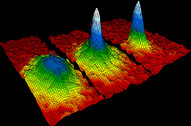
JILA の速度分布データ（左→右：冷却とともに中央へ凝縮体のピークが成長する）。

Velocity-distribution data from JILA (left to right: the condensate peak grows as the gas is cooled).

画像：Image: NIST/JILA/CU-Boulder — パブリックドメインpublic domain

なお、実験は調和トラップ中の気体です。凝縮の描像は共通ですが、転移温度や冪の具体式は、本文の一様気体とは異なります。

Note: the experiments are performed in a harmonic trap; the picture of condensation is the same, but the specific exponents and transition-temperature formula differ from the uniform gas of this note.

わずか4か月後、MIT のヴォルフガング・ケターレがナトリウム原子で桁違いに大きな凝縮体を実現します。のちに独立に用意した二つの凝縮体を重ねて干渉縞を観測し、凝縮体が巨視的な位相コヒーレンス——レーザー光のような「一つの物質波」性——をもつことを直接示しました。凝縮体をパルス状に取り出してみせる「原子レーザー」の実演もケターレのグループです。三人は2001年のノーベル物理学賞を受賞しました。

Only four months later Wolfgang Ketterle at MIT produced condensates of sodium atoms orders of magnitude larger. His group later overlapped two independently prepared condensates and observed interference fringes — direct evidence of macroscopic phase coherence, the matter-wave analogue of laser light — and demonstrated the pulsed "atom laser". The three shared the 2001 Nobel Prize in Physics.

以来、BEC は一度きりの珍品ではなく、現代物理の実験台になりました。渦糸を立てれば超流動が見え、光格子に載せれば多体模型をまるごと量子シミュレートできます。§5 で解いた理想ボース気体は、その世界へ入るための最初の地図です。

Since then the BEC has become not a one-off curiosity but a workbench of modern physics: stir it and vortices reveal superfluidity; load it into an optical lattice and it quantum-simulates whole many-body models. The ideal Bose gas solved in §5 is the first map into that world.

写真：Photos: Cornell (Betsythedevine, CC BY-SA 4.0) · Wieman (Christopher Michel, CC BY-SA 4.0) · Ketterle (Kzirkel, CC BY-SA 3.0) — Wikimedia Commons

6低温の三次元自由フェルミ粒子系The cold 3D free Fermi gas

次はフェルミ粒子系（\(\sigma=-1\)）です。中身は、ゾンマーフェルトが 1927 年の金属電子論で展開したもの。これにより金属電子の低温比熱が \(T\to0\) でゼロになることが説明され、当時の大問題が解決しました。

Now to fermions (\(\sigma=-1\)). The content is what Sommerfeld developed in his 1927 theory of metallic electrons; it explained why the low-temperature electronic heat capacity vanishes as \(T\to0\), resolving a major puzzle of the day.

6.1　フェルミ・エネルギーとフェルミ波数6.1　Fermi energy and Fermi wavenumber

絶対零度では、フェルミ分布は階段関数に潰れます：\(\bar n_{\mathrm F}(\varepsilon)\to\theta(\mu-\varepsilon)\)。エネルギー \(\varepsilon\le\mu\) の一粒子状態がびっしり詰まり、それ以上は空 —— フェルミ海です。\(T=0\) の化学ポテンシャルをフェルミ・エネルギー \(\varepsilon_{\mathrm F}\) と呼び、粒子数の条件 \(\displaystyle N=\int_0^{\varepsilon_{\mathrm F}}D(\varepsilon)\,d\varepsilon\)（\(\eqref{eq:NUint}\) の \(T\to0\) 極限）から決まります。\(D=A\sqrt{\varepsilon}\)（\(A\) は \(\eqref{eq:dos}\) の係数）を代入して積分すると

At absolute zero the Fermi distribution collapses to a step, \(\bar n_{\mathrm F}(\varepsilon)\to\theta(\mu-\varepsilon)\): every state with \(\varepsilon\le\mu\) is filled, all above are empty — the Fermi sea. The \(T=0\) chemical potential is the Fermi energy \(\varepsilon_{\mathrm F}\), fixed by \(\displaystyle N=\int_0^{\varepsilon_{\mathrm F}}D(\varepsilon)\,d\varepsilon\) (the \(T\to0\) limit of \(\eqref{eq:NUint}\)). Inserting \(D=A\sqrt{\varepsilon}\) (with the coefficient \(A\) of \(\eqref{eq:dos}\)) and integrating,

\(A=\dfrac{g\,V}{4\pi^{2}}\left(\dfrac{2m}{\hbar^{2}}\right)^{3/2}\) を戻すと \(\dfrac{3N}{2A}=\dfrac{6\pi^{2}N}{g\,V}\left(\dfrac{\hbar^{2}}{2m}\right)^{3/2}\) なので、

Restoring \(A=\dfrac{g\,V}{4\pi^{2}}\left(\dfrac{2m}{\hbar^{2}}\right)^{3/2}\) gives \(\dfrac{3N}{2A}=\dfrac{6\pi^{2}N}{g\,V}\left(\dfrac{\hbar^{2}}{2m}\right)^{3/2}\), hence

\(k_{\mathrm F}\) はフェルミ波数で、絶対零度では \(k\le k_{\mathrm F}\) の状態がすべて占有された球（フェルミ球）が実現します。スピン \(\dfrac12\) では \(g=2\) を入れて \(\varepsilon_{\mathrm F}=\dfrac{\hbar^{2}}{2m}(3\pi^{2}n)^{2/3}\)、\(k_{\mathrm F}=(3\pi^2n)^{1/3}\)。フェルミ温度 \(T_{\mathrm F}\equiv\dfrac{\varepsilon_{\mathrm F}}{k_{\mathrm B}}\) は \(T^{*}\) と同オーダー（\(\varepsilon_{\mathrm F}=1.21\,k_{\mathrm B}T^{*}\)）で、金属電子では \(10^4\,\mathrm{K}\) 程度、液体 \(^3\mathrm{He}\) では数 \(\mathrm{K}\) です。便利な等式として \(D(\varepsilon_{\mathrm F})=\dfrac{3}{2}\,\dfrac{N}{\varepsilon_{\mathrm F}}\)。

\(k_{\mathrm F}\) is the Fermi wavenumber: at \(T=0\) all states with \(k\le k_{\mathrm F}\) form a filled sphere (the Fermi sphere). For spin \(\dfrac12\), \(g=2\) gives \(\varepsilon_{\mathrm F}=\dfrac{\hbar^{2}}{2m}(3\pi^{2}n)^{2/3}\), \(k_{\mathrm F}=(3\pi^2n)^{1/3}\). The Fermi temperature \(T_{\mathrm F}\equiv\dfrac{\varepsilon_{\mathrm F}}{k_{\mathrm B}}\) is of the same order as \(T^{*}\) (\(\varepsilon_{\mathrm F}=1.21\,k_{\mathrm B}T^{*}\)): about \(10^4\,\mathrm{K}\) for metallic electrons, a few \(\mathrm{K}\) for liquid \(^3\mathrm{He}\). A handy identity is \(D(\varepsilon_{\mathrm F})=\dfrac{3}{2}\,\dfrac{N}{\varepsilon_{\mathrm F}}\).

ここで単位の感覚をひとつ。エネルギーを \(k_{\mathrm B}\) で割って温度に換算すると \(1\,\mathrm{eV}\approx1.16\times10^{4}\,\mathrm{K}\)（約 11600 K）。逆に室温 \(300\,\mathrm{K}\) は \(k_{\mathrm B}T\approx26\,\mathrm{meV}\)、つまり約 \(\dfrac{1}{40}\,\mathrm{eV}\) です。銅の伝導電子では \(\varepsilon_{\mathrm F}\approx7\,\mathrm{eV}\)、温度に直すと \(T_{\mathrm F}\approx8\times10^{4}\,\mathrm{K}\)——室温はその \(0.4\,\%\) にすぎません。電子にとって、室温は途方もない極低温なのです。金属の電子は日常のあらゆる温度でフェルミ縮退の底に沈んでいて（室温の銅で \(\mu\) のずれは \(\varepsilon_{\mathrm F}\) の \(10\) 万分の \(1\) 程度）、だからこそ、続く 6.2 の「低温展開」が金属のごく普通の室温物理をそのまま記述します。

A feel for the units: dividing by \(k_{\mathrm B}\), \(1\,\mathrm{eV}\approx1.16\times10^{4}\,\mathrm{K}\) (about 11,600 K); conversely room temperature, \(300\,\mathrm{K}\), is \(k_{\mathrm B}T\approx26\,\mathrm{meV}\approx\dfrac{1}{40}\,\mathrm{eV}\). For the conduction electrons of copper \(\varepsilon_{\mathrm F}\approx7\,\mathrm{eV}\), i.e. \(T_{\mathrm F}\approx8\times10^{4}\,\mathrm{K}\) — room temperature is a mere \(0.4\%\) of it. To the electrons, room temperature is fantastically cold. The electrons of a metal sit at the bottom of Fermi degeneracy at all everyday temperatures (in copper at 300 K the shift of \(\mu\) is about one part in \(10^{5}\) of \(\varepsilon_{\mathrm F}\)), which is exactly why the "low-temperature" expansion of 6.2 describes the perfectly ordinary room-temperature physics of metals.

6.2　ゾンマーフェルト展開6.2　The Sommerfeld expansion

低温では、フェルミ分布は \(\varepsilon=\mu\) のごく近く（幅 \(\sim k_{\mathrm B}T\)）でしか階段関数からずれません。この事実を、滑らかな関数 \(g(\varepsilon)\) に対する積分を系統的に評価する道具に仕立てます。まず、積分を「\(T=0\) の階段の寄与」と「そこからのずれ \(\Delta I\)」に分けます：

At low temperature the Fermi distribution departs from the step function only within a shell of width \(\sim k_{\mathrm B}T\) around \(\varepsilon=\mu\). Let us turn this fact into a systematic tool for integrals of a smooth \(g(\varepsilon)\). First split off the \(T=0\) step contribution, calling the rest \(\Delta I\):

角括弧の中身は \(\varepsilon=\mu\) の近くでしか値を持ちません。\(\varepsilon\gt\mu\) では \(\theta=0\) なので中身は \(\bar n_{\mathrm F}\) そのもの、\(\varepsilon\lt\mu\) では \(\theta=1\) なので \(\bar n_{\mathrm F}-1\) です。後者には恒等式

The bracket is nonzero only near \(\varepsilon=\mu\): above \(\mu\) (where \(\theta=0\)) it is just \(\bar n_{\mathrm F}\); below \(\mu\) (where \(\theta=1\)) it is \(\bar n_{\mathrm F}-1\), for which we use the identity

が使えます（分子分母に \(e^{-(\varepsilon-\mu)/k_{\mathrm B}T}\) を掛ければ一行で確かめられます）。つまり \(\mu\) の下側のずれも、上側と同じ「フェルミ関数の形」で書けます。積分を \(\varepsilon=\mu\) で二つに割り、下側で \(\varepsilon=\mu-k_{\mathrm B}T\,x\)、上側で \(\varepsilon=\mu+k_{\mathrm B}T\,x\) と置換すると、

(multiply numerator and denominator by \(e^{-(\varepsilon-\mu)/k_{\mathrm B}T}\) to check in one line). So the deviation below \(\mu\) takes the same Fermi-function shape as above. Cut the integral at \(\varepsilon=\mu\) and substitute \(\varepsilon=\mu-k_{\mathrm B}T\,x\) below and \(\varepsilon=\mu+k_{\mathrm B}T\,x\) above:

第一項の積分上限は本来 \(\dfrac{\mu}{k_{\mathrm B}T}\) ですが、被積分関数は \(e^{-x}\) で潰れるので、低温（\(\dfrac{\mu}{k_{\mathrm B}T}\gg1\)）では上限を \(\infty\) に伸ばしても誤差は \(e^{-\frac{\mu}{k_{\mathrm B}T}}\) 程度——これから拾うどの冪の項よりも小さい、指数関数的に小さい誤差です。伸ばしてしまえば二つの積分が同じ形にそろい、

The first integral really stops at \(\dfrac{\mu}{k_{\mathrm B}T}\), but the integrand dies off like \(e^{-x}\), so at low temperature (\(\dfrac{\mu}{k_{\mathrm B}T}\gg1\)) extending the limit to \(\infty\) costs only \(\sim e^{-\frac{\mu}{k_{\mathrm B}T}}\) — exponentially small, below every power we are about to keep. With both limits at \(\infty\) the two integrals combine:

ここが一番きれいなところです。分子は \(y=k_{\mathrm B}T\,x\) について \(g(\mu+y)-g(\mu-y)\) という奇関数なので、テイラー展開すると偶数階微分がすべて相殺し、奇数階だけが生き残ります：

Here comes the prettiest step. As a function of \(y=k_{\mathrm B}T\,x\), the numerator \(g(\mu+y)-g(\mu-y)\) is odd, so in its Taylor expansion every even derivative cancels and only odd ones survive:

（三次の係数は \(\dfrac{2}{3!}=\dfrac{1}{3}\) です。）これを代入すると、\(g\) に依存する部分・温度・普遍的な数値が綺麗に分離します：

(the cubic coefficient is \(\dfrac{2}{3!}=\dfrac{1}{3}\)). Substituting, the \(g\)-dependence, the temperature, and universal numbers separate cleanly:

（\(J_n\) はフェルミ型の定積分で、§7.5 で計算します。結果は \(J_n=(1-2^{1-n})\,\zeta(n)\,\Gamma(n)\)、特に \(J_2=\dfrac{\pi^2}{12}\)、\(J_4=\dfrac{7\pi^4}{120}\) です。）

(\(J_n\) is a Fermi-type definite integral, evaluated in §7.5: \(J_n=(1-2^{1-n})\,\zeta(n)\,\Gamma(n)\), in particular \(J_2=\dfrac{\pi^2}{12}\) and \(J_4=\dfrac{7\pi^4}{120}\).)

\(2J_2=\dfrac{\pi^2}{6}\)、\(\dfrac{J_4}{3}=\dfrac{7\pi^4}{360}\) を入れて、まとめます：

Inserting \(2J_2=\dfrac{\pi^2}{6}\) and \(\dfrac{J_4}{3}=\dfrac{7\pi^4}{360}\), we assemble the result:

これがゾンマーフェルト展開——低温フェルミ粒子系の万能道具です。補正が \(\left(\dfrac{k_{\mathrm B}T}{\mu}\right)^{\!2}\) の冪で入ること、そして 6.1 で見たとおり金属では室温でさえこの比が \(10^{-2}\) 程度であることを合わせると、この展開の強力さがわかります。

This is the Sommerfeld expansion — the workhorse of the cold Fermi gas. Its corrections enter as powers of \(\left(\dfrac{k_{\mathrm B}T}{\mu}\right)^{\!2}\); recalling from 6.1 that in a metal this ratio is only \(\sim10^{-2}\) even at room temperature, you see how powerful the expansion is.

6.3　低温の化学ポテンシャルと比熱6.3　Cold chemical potential and heat capacity

手順は決まっています。粒子数一定の条件 \(\eqref{eq:NUint}\) は有限温度でも成り立ちます：\(\displaystyle N=\int_0^{\infty}D(\varepsilon)\,\bar n_{\mathrm F}(\varepsilon)\,d\varepsilon\)。これはゾンマーフェルト展開 \(\eqref{eq:sommer}\) の \(g(\varepsilon)=D(\varepsilon)=A\sqrt{\varepsilon}\) の場合です。\(g'(\mu)=\dfrac{A}{2\sqrt{\mu}}\) に注意して \(T^{2}\) まで拾うと、

The procedure is fixed. The particle-number condition \(\eqref{eq:NUint}\) holds at finite temperature too: \(\displaystyle N=\int_0^{\infty}D(\varepsilon)\,\bar n_{\mathrm F}(\varepsilon)\,d\varepsilon\). This is the Sommerfeld expansion \(\eqref{eq:sommer}\) with \(g(\varepsilon)=D(\varepsilon)=A\sqrt{\varepsilon}\). Noting \(g'(\mu)=\dfrac{A}{2\sqrt{\mu}}\) and keeping terms to \(T^{2}\),

左辺の \(N\) は 6.1 の \(T=0\) の関係 \(N=\dfrac{2}{3}A\,\varepsilon_{\mathrm F}^{3/2}\) と同じものです。等しいと置いて \(\dfrac{2}{3}A\) を払うと、

The \(N\) on the left is the same as the \(T=0\) relation of 6.1, \(N=\dfrac{2}{3}A\,\varepsilon_{\mathrm F}^{3/2}\). Equating the two and cancelling \(\dfrac{2}{3}A\),

右辺の補正はすでに \(\left(\dfrac{k_{\mathrm B}T}{\mu}\right)^{\!2}\) の小ささを持つので、その中では0次の \(\mu\approx\varepsilon_{\mathrm F}\) を使って構いません。\((1+x)^{-2/3}=1-\dfrac{2}{3}x+O(x^{2})\) を当てて、

The correction on the right is already small, of order \(\left(\dfrac{k_{\mathrm B}T}{\mu}\right)^{\!2}\), so inside it we may use the zeroth-order \(\mu\approx\varepsilon_{\mathrm F}\). Applying \((1+x)^{-2/3}=1-\dfrac{2}{3}x+O(x^{2})\),

化学ポテンシャルは温度とともにわずかに下がる——図 1 の \(\mu\) のフェルミ曲線の出だしです。次に内部エネルギー。\(\eqref{eq:NUint}\) の \(U\) は \(\eqref{eq:sommer}\) の \(g(\varepsilon)=A\varepsilon^{3/2}\)（\(g'(\mu)=\dfrac{3}{2}A\sqrt{\mu}\)）の場合なので、

The chemical potential thus drifts slightly downward with temperature — the start of the Fermi \(\mu\)-curve in Fig. 1. Next the internal energy: the \(U\) of \(\eqref{eq:NUint}\) is the case \(g(\varepsilon)=A\varepsilon^{3/2}\) of \(\eqref{eq:sommer}\) (so \(g'(\mu)=\dfrac{3}{2}A\sqrt{\mu}\)):

ここに、いま求めた \(\mu(T)\) を代入します。\((1+x)^{5/2}=1+\dfrac{5}{2}x+O(x^{2})\) より \(\mu^{5/2}\approx\varepsilon_{\mathrm F}^{5/2}\bigl[1-\dfrac{5\pi^{2}}{24}\,t^{2}\bigr]\)（略記 \(t\equiv\dfrac{k_{\mathrm B}T}{\varepsilon_{\mathrm F}}\)）。二つの補正を合わせると、

Now insert the \(\mu(T)\) just found. From \((1+x)^{5/2}=1+\dfrac{5}{2}x+O(x^{2})\), \(\mu^{5/2}\approx\varepsilon_{\mathrm F}^{5/2}\bigl[1-\dfrac{5\pi^{2}}{24}\,t^{2}\bigr]\) (shorthand \(t\equiv\dfrac{k_{\mathrm B}T}{\varepsilon_{\mathrm F}}\)). Combining the two corrections,

途中で \(-\dfrac{5\pi^{2}}{24}+\dfrac{5\pi^{2}}{8}=\dfrac{5\pi^{2}}{12}\)（通分すると \(-\dfrac{1}{24}+\dfrac{3}{24}=\dfrac{2}{24}\)）、最後に 6.1 の \(N=\dfrac{2}{3}A\varepsilon_{\mathrm F}^{3/2}\) から \(\dfrac{2}{5}A\varepsilon_{\mathrm F}^{5/2}=\dfrac{3}{5}N\varepsilon_{\mathrm F}\) を使いました。\(T=0\) の値 \(U(0)=\dfrac{3}{5}N\varepsilon_{\mathrm F}\)——粒子あたり平均 \(\dfrac{3}{5}\varepsilon_{\mathrm F}\)——も同時に読み取れます。最後に \(T\) で微分すれば、

Here \(-\dfrac{5\pi^{2}}{24}+\dfrac{5\pi^{2}}{8}=\dfrac{5\pi^{2}}{12}\) (over a common denominator, \(-\dfrac{1}{24}+\dfrac{3}{24}=\dfrac{2}{24}\)), and in the last step \(N=\dfrac{2}{3}A\varepsilon_{\mathrm F}^{3/2}\) of 6.1 gives \(\dfrac{2}{5}A\varepsilon_{\mathrm F}^{5/2}=\dfrac{3}{5}N\varepsilon_{\mathrm F}\). The zero-temperature value \(U(0)=\dfrac{3}{5}N\varepsilon_{\mathrm F}\) — an average of \(\dfrac{3}{5}\varepsilon_{\mathrm F}\) per particle — can be read off as well. Finally, differentiate in \(T\):

最後の等号では 6.1 の \(D(\varepsilon_{\mathrm F})=\dfrac{3N}{2\varepsilon_{\mathrm F}}\) を使いました。まとめると：

where the last equality used \(D(\varepsilon_{\mathrm F})=\dfrac{3N}{2\varepsilon_{\mathrm F}}\) of 6.1. In summary:

コラム：ゾンマーフェルトと「比熱の謎」Column: Sommerfeld and the heat-capacity puzzleクリックで展開click to expand

A. Sommerfeld

1868–1951

金属の電気は自由な電子が運ぶ——1900年のドルーデ模型は電気伝導をみごとに説明しましたが、致命的な矛盾を一つ抱えていました。電子が古典気体なら、比熱に一粒子あたり \(\dfrac32 k_{\mathrm B}\)（§4 の古典値）を上乗せするはずです。ところが実測の金属比熱に、電子の寄与はほとんど見えない。電気は運ぶのに、熱は受け取らない？——これが四半世紀つづいた「比熱の謎」です。

Free electrons carry a metal's electricity — the Drude model of 1900 explained conduction beautifully, yet it hid a fatal contradiction. A classical electron gas should add \(\dfrac32 k_{\mathrm B}\) per particle to the heat capacity (the classical value of §4); the measured heat capacity of metals shows almost no electronic contribution. They carry charge but accept no heat? That "heat-capacity puzzle" stood for a quarter of a century.

答えは、いま 6.3 で出ました。\(C\propto T\) が言うとおり、熱を受け取れるのはフェルミ面近傍の幅 \(k_{\mathrm B}T\) にいる電子だけ——室温では全体の 1% 足らずです。古典値より2桁小さく、格子振動の比熱に埋もれて見えなかったのです。1927年、発表されたばかりのフェルミ統計をドルーデ模型に組み込み、これを示したのがゾンマーフェルトでした。

The answer is the one just derived in 6.3. As \(C\propto T\) says, only electrons within \(k_{\mathrm B}T\) of the Fermi surface can accept heat — at room temperature, well under 1% of them. Two orders of magnitude below the classical value, the electronic term hides beneath the lattice contribution. Sommerfeld showed this in 1927 by wiring the brand-new Fermi statistics into the Drude model.

ゾンマーフェルト自身は、ノーベル賞に80回以上ノミネートされて一度も受賞しなかった記録の持ち主です。そのかわり——と言うべきか——彼のミュンヘンの教室からは、ハイゼンベルク、パウリ、デバイ、ベーテと、博士学生だけで4人のノーベル賞受賞者が巣立ちました。アインシュタインは手紙で、若い才能を「土の中から掘り起こす」その手腕を称えたと伝えられています。誰にでも毒舌だったパウリが、生涯頭の上がらなかった数少ない相手だったとも伝えられています。

Sommerfeld himself holds a bittersweet record: nominated for the Nobel Prize more than 80 times, he never won. Instead, his Munich seminar raised four Nobel laureates among his doctoral students alone — Heisenberg, Pauli, Debye, Bethe. Einstein is said to have praised, in a letter, his knack for "digging young talents out of the soil"; and Pauli, whose sharp tongue spared no one, is said to have deferred to Sommerfeld alone all his life.

写真：Photo: Sommerfeld (1897) — Wikimedia Commons（パブリックドメイン） (public domain)

コラム：白色矮星——絶対零度の圧力が星を支えるColumn: white dwarfs — pressure at absolute zero holds up a starクリックで展開click to expand

S. Chandrasekhar

1910–1995

シリウスの伴星シリウス B は、太陽なみの質量が地球サイズに詰め込まれた星です。平均密度はおよそ \(2\times10^{9}\,\mathrm{kg/m^{3}}\)——角砂糖ひとつぶんで約2トン。この異常な星を支える力の正体を、フェルミ統計の登場からわずか数か月後の1926年末、R. H. ファウラーが見抜きました。縮退圧——パウリの排他原理が生む、低温では温度にほとんど依存せず、絶対零度でも残る圧力です。

Sirius B, the companion of Sirius, packs roughly a solar mass into an Earth-sized ball: mean density about \(2\times10^{9}\,\mathrm{kg/m^{3}}\) — a sugar cube weighing some two tonnes. What holds such a star up was identified at the end of 1926, months after Fermi statistics appeared, by R. H. Fowler: degeneracy pressure — a pressure born of Pauli exclusion that survives even at absolute zero and, at low temperature, hardly depends on temperature at all.

非相対論的な第一近似では、中身は §6 の式です。3.3 の \(PV=\dfrac23 U\) と 6.3 の \(U(0)=\dfrac35 N\varepsilon_{\mathrm F}\) を合わせると、\(T=0\) でも圧力 \(P=\dfrac25 n\varepsilon_{\mathrm F}\) が残ります。白色矮星の電子密度 \(n\sim10^{36}\,\mathrm{m^{-3}}\) ではフェルミ温度は \(T_{\mathrm F}\sim3\times10^{9}\,\mathrm K\)。中心温度は \(10^{7}\,\mathrm K\) もありますが、比を取れば \(\dfrac{T}{T_{\mathrm F}}\sim0.3\,\%\)——室温の銅（0.4%）より「低温」です。星の質量は炭素や酸素の原子核が担い、圧力は縮退電子が担う——その電子系が、まるごと §6 の縮退フェルミ気体なのです。

In the non-relativistic first approximation, the physics is that of §6. Combining \(PV=\dfrac23 U\) of 3.3 with \(U(0)=\dfrac35 N\varepsilon_{\mathrm F}\) of 6.3 leaves a pressure \(P=\dfrac25 n\varepsilon_{\mathrm F}\) even at \(T=0\). At the white-dwarf electron density \(n\sim10^{36}\,\mathrm{m^{-3}}\) the Fermi temperature is \(T_{\mathrm F}\sim3\times10^{9}\,\mathrm K\); the core may reach \(10^{7}\,\mathrm K\), yet \(\dfrac{T}{T_{\mathrm F}}\sim0.3\,\%\) — "colder" than room-temperature copper (0.4%). The carbon and oxygen nuclei carry the star's mass; the degenerate electrons carry its pressure — and that electron gas is exactly the Fermi gas of §6.

1930年、19歳のチャンドラセカールは、インドから英国へ向かう船上でこの理論を相対論へ拡張します。密度が上がって \(\varepsilon_{\mathrm F}\) が電子の静止エネルギー \(m_{e}c^{2}=0.51\,\mathrm{MeV}\) に近づくと（シリウス B の平均密度から非相対論式で見積もると、すでに半分ほど）、\(\varepsilon\approx pc\) となって圧力は \(P\propto n^{5/3}\) から \(P\propto n^{4/3}\) へ弱まり、重力とちょうど同じスケーリングになる——つまり約1.4太陽質量を超えると、縮退圧では支えきれない。このチャンドラセカール限界は、白色矮星の熱核暴走である Ia 型超新星を理解する鍵となり、また大質量星の中心核がこの限界を超えて崩壊する先には中性子星が待っています。53年後の1983年、ノーベル賞で報われました。

In 1930 the 19-year-old Chandrasekhar, on the boat from India to England, made the theory relativistic. As density grows and \(\varepsilon_{\mathrm F}\) approaches the electron rest energy \(m_{e}c^{2}=0.51\,\mathrm{MeV}\) (a nonrelativistic estimate at Sirius B's mean density already puts it about halfway there), \(\varepsilon\approx pc\) softens the pressure from \(P\propto n^{5/3}\) to \(P\propto n^{4/3}\) — precisely gravity's scaling. Beyond about 1.4 solar masses, degeneracy pressure loses. The Chandrasekhar limit became the key to type-Ia supernovae (the thermonuclear runaway of a white dwarf), and — via the collapse of massive stellar cores that exceed it — to neutron stars; it was rewarded with the Nobel Prize 53 years later, in 1983.

写真：Photo: Chandrasekhar（NASA）— Wikimedia Commons（パブリックドメイン） (public domain)

7物理数学のまとめMathematical appendix

本文で使った数学のうち、流れを止めたくなくて後回しにした細部をここに集めました。必要になったときに戻ってくるための章です。

Here we collect the mathematical details that were deferred so as not to interrupt the flow of the main text — a chapter to come back to when needed.

7.1　ガンマ関数の振り返り7.1　A quick review of the gamma function

ガンマ関数は次の積分で定義されます（\(\nu\gt0\)）：

The gamma function is defined by the integral (\(\nu\gt0\)):

一番大事な性質は漸化式です。部分積分で一行：

Its most important property is the recursion, one line by integration by parts:

\(\displaystyle\Gamma(1)=\int_0^\infty e^{-t}dt=1\) なので、正の整数では \(\Gamma(n+1)=n!\)——ガンマ関数は階乗の連続化です。半整数の出発点は \(\Gamma\!\left(\dfrac{1}{2}\right)\) で、\(t=u^2\)（\(dt=2u\,du\)）と置換するとガウス積分に化けます：

Since \(\displaystyle\Gamma(1)=\int_0^\infty e^{-t}dt=1\), for positive integers \(\Gamma(n+1)=n!\) — the gamma function extends the factorial. The half-integer seed is \(\Gamma\!\left(\dfrac{1}{2}\right)\): substituting \(t=u^2\) (\(dt=2u\,du\)) turns it into the Gaussian integral:

漸化式と合わせると、本文で使った二つの値が出ます：

Combined with the recursion, this yields the two values used in the main text:

もう一つ、置換 \(t=kx\) から従う「働き者」の公式を挙げておきます：

One more workhorse formula, following from the substitution \(t=kx\):

（この公式が、次の 7.2 と、§5・§6 に現れるゼータ関数がらみの定積分すべての土台になります。）

(This formula underlies 7.2 below, as well as every zeta-related definite integral of §5 and §6.)

7.2　\(\varphi_\nu\) の積分表示と級数表示は一致する7.2　The integral and series forms of \(\varphi_\nu\) agree

定義 \(\eqref{eq:phinu}\) の二つの表示が等しいことを、途中を飛ばさずに確かめます。出発点は積分表示：

We verify, without skipping a step, that the two forms in the definition \(\eqref{eq:phinu}\) agree. The starting point is the integral form:

まず分母を等比級数にほどきます（\(|z e^{-x}|\lt1\) のとき）：

First unravel the denominator into a geometric series (valid for \(|z e^{-x}|\lt1\)):

これを積分表示に代入して項別に積分し、7.1 の公式 \(\displaystyle\int_0^{\infty}x^{\nu-1}e^{-kx}\,dx=\dfrac{\Gamma(\nu)}{k^{\nu}}\) を各項に当てると、先頭の \(\dfrac{1}{\Gamma(\nu)}\) と打ち消し合って

Insert this into the integral form, integrate term by term, and apply the formula of 7.1, \(\displaystyle\int_0^{\infty}x^{\nu-1}e^{-kx}\,dx=\dfrac{\Gamma(\nu)}{k^{\nu}}\), to each term; the prefactor \(\dfrac{1}{\Gamma(\nu)}\) cancels and

項別積分が正当化できるのは、級数が絶対収束する範囲です。級数表示は \(|z|\lt1\) で絶対収束し、境界 \(|z|=1\) でも \(\nu\gt1\) なら絶対収束します——本文で用いる \(\nu=\dfrac32,\dfrac52\) はこれに該当します。低温フェルミ気体の \(z\gt1\) では級数表示は使えないため、積分表示を用います（そちらが \(\varphi_\nu\) の定義。3.4 の注意と整合しています）。

Term-by-term integration is justified where the series converges absolutely. The series representation converges absolutely for \(|z|\lt1\); on the boundary \(|z|=1\) it still converges absolutely whenever \(\nu\gt1\), which covers the \(\nu=\dfrac32,\dfrac52\) used in this note. For the cold Fermi gas, \(z\gt1\), the series is unavailable and the integral representation — the definition of \(\varphi_\nu\) — takes over, in exact agreement with the caveat of 3.4.

7.3　ボース型定積分と \(\varphi_\nu(1)=\zeta(\nu)\)7.3　The Bose-type integral and \(\varphi_\nu(1)=\zeta(\nu)\)

§5 で使うボース型の定積分は、7.2 と同じように分母を級数にほどくだけで計算できます。分母が \(e^{x}-1\) なら級数の符号はすべて正で、 \(\displaystyle\frac{1}{e^{x}-1}=\frac{e^{-x}}{1-e^{-x}}=\sum_{k=1}^{\infty}e^{-kx}\) をそのまま使い、各項に 7.1 の公式を当てるだけです：

The Bose-type integral used in §5 is computed just as in 7.2, by unravelling the denominator into a series. With \(e^{x}-1\) every sign comes out positive: use \(\displaystyle\frac{1}{e^{x}-1}=\frac{e^{-x}}{1-e^{-x}}=\sum_{k=1}^{\infty}e^{-kx}\) and apply the formula of 7.1 to each term:

右の同値は、\(\varphi_\nu\) の定義 \(\eqref{eq:phinu}\) で \(z=1\)（\(\sigma=+1\)）と置いたものです。これが 5.1・5.2 で使った \(\varphi_{3/2}(1)=\zeta\!\left(\dfrac{3}{2}\right)=2.612\cdots\)、\(\varphi_{5/2}(1)=\zeta\!\left(\dfrac{5}{2}\right)=1.341\cdots\) の出どころ——「\(\varphi_\nu(1)\) は積分表示でも級数表示でも同じ \(\zeta(\nu)\) になる」というだけのことです。

The equivalence on the right is just the definition \(\eqref{eq:phinu}\) of \(\varphi_\nu\) at \(z=1\) (\(\sigma=+1\)). This is the origin of \(\varphi_{3/2}(1)=\zeta\!\left(\dfrac{3}{2}\right)=2.612\cdots\) and \(\varphi_{5/2}(1)=\zeta\!\left(\dfrac{5}{2}\right)=1.341\cdots\) used in 5.1 and 5.2 — simply the statement that \(\varphi_\nu(1)\) equals the same \(\zeta(\nu)\) whether you read it as an integral or a series.

7.4　\(z\to1\) の平方根特異性（ロビンソン展開）7.4　The square-root singularity at \(z\to1\) (Robinson expansion)

5.3 で使った展開 \(\varphi_{3/2}(e^{-\alpha})=\zeta\!\left(\dfrac{3}{2}\right)-2\sqrt{\pi\alpha}+O(\alpha)\)（\(\alpha\gt0\) は小さい）を導きます。出発点は級数 \(\eqref{eq:phinu}\)。\(z=e^{-\alpha}\) を入れ、\(\alpha=0\) の値 \(\zeta\!\left(\dfrac{3}{2}\right)\) との差を取ります：

We derive the expansion used in 5.3, \(\varphi_{3/2}(e^{-\alpha})=\zeta\!\left(\dfrac{3}{2}\right)-2\sqrt{\pi\alpha}+O(\alpha)\) for small \(\alpha\gt0\). Start from the series \(\eqref{eq:phinu}\) with \(z=e^{-\alpha}\), and subtract the \(\alpha=0\) value \(\zeta\!\left(\dfrac{3}{2}\right)\):

分子 \(e^{-\alpha k}-1\) が効き始めるのは \(k\sim\dfrac{1}{\alpha}\gg1\) の遠方です。和の刻み幅 \(1\) はこのスケールに比べて十分細かいので、3.2 のコラムとまったく同じ理屈（リーマン和）で、和を積分に置き換えられます：

The numerator \(e^{-\alpha k}-1\) switches on only at \(k\sim\dfrac{1}{\alpha}\gg1\), far out where the unit spacing of the sum is fine compared with the relevant scale. By exactly the Riemann-sum logic of the column in 3.2, the sum may be replaced by an integral:

二つ目の等号は置換 \(t=\dfrac{u}{\alpha}\) です（\(t^{-3/2}dt=\alpha^{1/2}u^{-3/2}du\)——ここで \(\sqrt{\alpha}\) が生まれます）。積分自体は \(0\) でも \(\infty\) でも収束しています：\(u\to0\) で被積分関数は \(-u^{-1/2}\)、\(u\to\infty\) で \(-u^{-3/2}\) 程度だからです。値は部分積分一発で出ます。\(u^{-3/2}du=d(-2u^{-1/2})\) と見て、

the second equality being the substitution \(t=\dfrac{u}{\alpha}\) (so \(t^{-3/2}dt=\alpha^{1/2}u^{-3/2}du\) — this is where the \(\sqrt{\alpha}\) is born). The integral converges at both ends: the integrand behaves like \(-u^{-1/2}\) as \(u\to0\) and like \(-u^{-3/2}\) as \(u\to\infty\). One integration by parts, reading \(u^{-3/2}du=d(-2u^{-1/2})\), evaluates it:

境界項は \(u\to0\) で \(-2u^{-1/2}(e^{-u}-1)\approx2u^{1/2}\to0\)、\(u\to\infty\) で \(2u^{-1/2}\to0\) と、両端で消えます。最後は 7.1 の \(\Gamma\!\left(\dfrac{1}{2}\right)=\sqrt{\pi}\) です。まとめると、

both boundary terms vanish (\(-2u^{-1/2}(e^{-u}-1)\approx2u^{1/2}\to0\) as \(u\to0\); \(2u^{-1/2}\to0\) as \(u\to\infty\)), and the last step is \(\Gamma\!\left(\dfrac{1}{2}\right)=\sqrt{\pi}\) from 7.1. Altogether,

（\(\sqrt{\alpha}\) は \(\alpha\) で微分すると \(\alpha\to0\) で発散します——これが「\(z=1\) で微分不可能」の正体で、5.3 の \(\mu\propto(T-T_0)^{2}\) という振る舞いの源です。和→積分の置き換えで捨てた分は \(O(\alpha)\) 以降にしか効きません。）

(The derivative of \(\sqrt{\alpha}\) diverges as \(\alpha\to0\) — this is the precise sense in which \(\varphi_{3/2}\) is not differentiable at \(z=1\), and the source of the \(\mu\propto(T-T_0)^{2}\) behaviour of 5.3. What the sum-to-integral replacement discards only affects order \(\alpha\) and beyond.)

7.5　フェルミ型定積分 \(J_n\) とゼータ関数7.5　The Fermi-type integral \(J_n\) and the zeta function

6.2 のゾンマーフェルト展開に現れた定積分

We evaluate the definite integral that appeared in the Sommerfeld expansion of 6.2,

を計算します。手順は 7.3 のボース型とまったく同じで、分母を級数にほどいて項別に積分するだけです。ただし今回は分母が \(+1\) なので、交代級数になります（\(x\gt0\) で \(e^{-x}\lt1\) だから収束）：

The procedure is exactly that of the Bose case in 7.3: unravel the denominator into a series and integrate term by term — except that with a \(+1\) in the denominator the series alternates (convergent since \(e^{-x}\lt1\) for \(x\gt0\)):

7.1 の公式 \(\displaystyle\int_0^{\infty}x^{n-1}e^{-kx}\,dx=\dfrac{\Gamma(n)}{k^{n}}\) を各項に当てると、

Applying the formula of 7.1, \(\displaystyle\int_0^{\infty}x^{n-1}e^{-kx}\,dx=\dfrac{\Gamma(n)}{k^{n}}\), to each term,

残った交代級数を、リーマンのゼータ関数 \(\displaystyle\zeta(n)\equiv\sum_{k=1}^{\infty}\frac{1}{k^{n}}\) で表すのが最後の一手です。二つの級数を上下に並べて書いてみます。奇数の項はまったく同じで、偶数の項だけ符号が逆です：

The last move expresses the alternating sum through the Riemann zeta function \(\displaystyle\zeta(n)\equiv\sum_{k=1}^{\infty}\frac{1}{k^{n}}\). Write the two series one above the other: the odd terms are identical, and only the even terms flip sign:

上の行から下の行を引くと、奇数項は打ち消し合い、偶数項だけが \(\dfrac{2}{k^{n}}\) ずつ残ります。残った偶数項の分母を \(k=2m\)（\(m=1,2,3,\dots\)）と書き直すと、共通因子 \(2^{-n}\) がくくり出せて、全体がまた \(\zeta(n)\) になります：

Subtract the lower line from the upper: the odd terms cancel, and each even term survives with weight \(\dfrac{2}{k^{n}}\). Renaming the even denominators \(k=2m\) (\(m=1,2,3,\dots\)) pulls out a common factor \(2^{-n}\), and the sum becomes \(\zeta(n)\) again:

移項すれば、交代級数がゼータ関数だけで書けます：

Transposing gives the alternating series in terms of \(\zeta\) alone:

これを先ほどの \(J_n\) に戻せば：

Insert this back into \(J_n\):

本文で使う二つの値は、既知の \(\zeta(2)=\dfrac{\pi^{2}}{6}\)、\(\zeta(4)=\dfrac{\pi^{4}}{90}\)（バーゼル問題とその親戚）から：

The two values used in the main text follow from the classic results \(\zeta(2)=\dfrac{\pi^{2}}{6}\) and \(\zeta(4)=\dfrac{\pi^{4}}{90}\) (the Basel problem and its cousin):

コラム：バーゼル問題とその親戚 —— \(\sin x\) を因数分解するColumn: the Basel problem and its cousins — factorising \(\sin x\)クリックで展開click to expand

上で「既知の値」として使った \(\zeta(2)=\dfrac{\pi^{2}}{6}\) と \(\zeta(4)=\dfrac{\pi^{4}}{90}\) を最初に求めたのはオイラー（1735年）で、その導出は驚くほど単純です。まずウォームアップとして、多項式の因数定理を思い出します。3次多項式 \(p(x)\) の零点が \(x=0,\ +a,\ -a\) の三つで、しかも \(x\to0\) で \(p(x)\approx x\) だとわかっているなら、\(p(x)\) は

The values \(\zeta(2)=\dfrac{\pi^{2}}{6}\) and \(\zeta(4)=\dfrac{\pi^{4}}{90}\) quoted above were first obtained by Euler (1735), by an argument of striking simplicity. As a warm-up, recall the factor theorem for polynomials: if a cubic \(p(x)\) has zeros exactly at \(x=0,\ +a,\ -a\), and moreover \(p(x)\approx x\) as \(x\to0\), then

\[ p(x)=x\Bigl(1-\frac{x}{a}\Bigr)\Bigl(1+\frac{x}{a}\Bigr)=x\Bigl(1-\frac{x^{2}}{a^{2}}\Bigr) \]

と書けます。根 \(\pm a\) をペアで掛けると \(\left(1-\dfrac{x}{a}\right)\left(1+\dfrac{x}{a}\right)=1-\dfrac{x^{2}}{a^{2}}\) という「\(x^{2}\) だけの因子」になるのがポイントです（各因子を \(1-\cdots\) の形に整えておいたので、\(x\to0\) で全体がきちんと \(x\) に近づきます）。

The point is that multiplying the paired roots \(\pm a\) gives \(\left(1-\dfrac{x}{a}\right)\left(1+\dfrac{x}{a}\right)=1-\dfrac{x^{2}}{a^{2}}\), a factor containing only \(x^{2}\); and since each factor is normalised to the form \(1-\cdots\), the whole expression correctly approaches \(x\) as \(x\to0\).

では \(\sin x\) ではどうか。グラフを見ると、零点は \(x=0\) と \(x=\pm n\pi\)（\(n=1,2,3,\dots\)）に等間隔で並んでいて、それ以外にはありません：

Now, what about \(\sin x\)? Look at the graph: its zeros sit at \(x=0\) and \(x=\pm n\pi\) (\(n=1,2,3,\dots\)), equally spaced, and nowhere else:

そこでオイラーは、\(\sin x\) を「無限次の多項式」とみなし、上のウォームアップをそのまま無限個の根に延長しました。根 \(\pm n\pi\) をペアで括れば

Euler's move: treat \(\sin x\) as a "polynomial of infinite degree" and extend the warm-up to infinitely many roots. Pairing the roots \(\pm n\pi\),

\[ \sin x = x\Bigl(1-\frac{x^{2}}{\pi^{2}}\Bigr)\Bigl(1-\frac{x^{2}}{4\pi^{2}}\Bigr)\Bigl(1-\frac{x^{2}}{9\pi^{2}}\Bigr)\cdots = x\prod_{n=1}^{\infty}\Bigl(1-\frac{x^{2}}{n^{2}\pi^{2}}\Bigr). \]

各因子は \(x\to0\) で \(1\) に近づくので、右辺全体は \(x\to0\) で \(x\) に近づき、\(\sin x\approx x\) と整合しています（これが全体の定数を \(1\) に決めています）。

Each factor tends to \(1\) as \(x\to0\), so the right-hand side tends to \(x\), consistent with \(\sin x\approx x\) — this is what fixes the overall constant to \(1\).

次に、この積を展開したときに \(x^{2}\) と \(x^{4}\) の係数がどう出るかを、まず因子3個で確かめます。\(a_{n}\) を小さな数として

Next, let us see how the coefficients of \(x^{2}\) and \(x^{4}\) arise when the product is expanded — first with just three factors. With small numbers \(a_{n}\),

\[ (1-a_{1}x^{2})(1-a_{2}x^{2})(1-a_{3}x^{2}) =1-(a_{1}+a_{2}+a_{3})\,x^{2}+(a_{1}a_{2}+a_{1}a_{3}+a_{2}a_{3})\,x^{4}-a_{1}a_{2}a_{3}\,x^{6}. \]

\(x^{2}\) の項は「どれか一つの括弧から \(-a_{k}x^{2}\) を拾い、残りからは \(1\) を拾う」ことで生まれるので、係数は \(-\sum_k a_{k}\)。\(x^{4}\) の項は「二つの括弧から拾う」ので、異なるペアにわたる和 \(\sum_{m\lt n}a_{m}a_{n}\) が立ちます。この数え方は因子が無限個でも変わりません。そこで \(a_{n}=\dfrac{1}{n^{2}\pi^{2}}\) と置いて両辺を \(x\) で割ると

The \(x^{2}\) term arises by picking \(-a_{k}x^{2}\) from one bracket and \(1\) from all the others, so its coefficient is \(-\sum_k a_{k}\); the \(x^{4}\) term picks from two brackets, giving the sum over distinct pairs \(\sum_{m\lt n}a_{m}a_{n}\). The same counting works for infinitely many factors. Setting \(a_{n}=\dfrac{1}{n^{2}\pi^{2}}\) and dividing by \(x\),

\[ \frac{\sin x}{x} = 1-\Bigl(\sum_{n=1}^{\infty}\frac{1}{n^{2}\pi^{2}}\Bigr)x^{2} +\Bigl(\sum_{m\lt n}\frac{1}{m^{2}n^{2}\pi^{4}}\Bigr)x^{4}-\cdots. \]

一方、おなじみのテイラー展開 \(\sin x=x-\dfrac{x^{3}}{3!}+\dfrac{x^{5}}{5!}-\cdots\) を \(x\) で割れば

On the other hand, dividing the familiar Taylor series \(\sin x=x-\dfrac{x^{3}}{3!}+\dfrac{x^{5}}{5!}-\cdots\) by \(x\),

\[ \frac{\sin x}{x}=1-\frac{x^{2}}{6}+\frac{x^{4}}{120}-\cdots. \]

同じ関数を二通りに書いたのだから、係数は一致しなければなりません。\(x^{2}\) の係数の比較から

These are two expressions for the same function, so the coefficients must match. Comparing the coefficients of \(x^{2}\):

\[ \sum_{n=1}^{\infty}\frac{1}{n^{2}\pi^{2}}=\frac{1}{6} \quad\Longrightarrow\quad \zeta(2)=\sum_{n=1}^{\infty}\frac{1}{n^{2}}=\frac{\pi^{2}}{6}=1.6449\dots \]

（両辺に \(\pi^{2}\) を掛けただけです。）「平方数の逆数をぜんぶ足すといくつか」というバーゼル問題の答えが、こんなに短い道のりで出ました。\(x^{4}\) の係数の比較も同様に、両辺に \(\pi^{4}\) を掛けて

(just multiply both sides by \(\pi^{2}\)). That settles the Basel problem — "what is the sum of the reciprocals of the squares?" — in remarkably few steps. Comparing the coefficients of \(x^{4}\) and multiplying by \(\pi^{4}\) likewise gives

\[ \sum_{m\lt n}\frac{1}{m^{2}n^{2}\pi^{4}}=\frac{1}{120} \quad\Longrightarrow\quad \sum_{m\lt n}\frac{1}{m^{2}n^{2}}=\frac{\pi^{4}}{120}. \]

欲しいのは対角の和 \(\zeta(4)=\sum_n \dfrac{1}{n^{4}}\) であって、この「ペアの和」ではありません。両者をつなぐのが、二乗の展開です。因子3個で書けば

What we want, though, is the diagonal sum \(\zeta(4)=\sum_n \dfrac{1}{n^{4}}\), not this pair sum. The bridge is the expansion of a square — with three terms,

\[ (a_{1}+a_{2}+a_{3})^{2} =\underbrace{a_{1}^{2}+a_{2}^{2}+a_{3}^{2}}_{\text{対角}} +\,2\,(\underbrace{a_{1}a_{2}+a_{1}a_{3}+a_{2}a_{3}}_{\text{ペア}}), \]

つまり一般に \(\Bigl(\sum_n \dfrac{1}{n^{2}}\Bigr)^{2}=\sum_n \dfrac{1}{n^{4}}+2\sum_{m\lt n}\dfrac{1}{m^{2}n^{2}}\)。これを \(\zeta(4)\) について解いて、いま求めた二つの値を代入します：

i.e. in general \(\Bigl(\sum_n \dfrac{1}{n^{2}}\Bigr)^{2}=\sum_n \dfrac{1}{n^{4}}+2\sum_{m\lt n}\dfrac{1}{m^{2}n^{2}}\). Solve for \(\zeta(4)\) and insert the two values just found:

\[ \zeta(4)=\Bigl(\frac{\pi^{2}}{6}\Bigr)^{2}-2\cdot\frac{\pi^{4}}{120} =\frac{\pi^{4}}{36}-\frac{\pi^{4}}{60} =\frac{5\pi^{4}-3\pi^{4}}{180} =\frac{\pi^{4}}{90}. \]

同じ手続きを \(x^{6},\ x^{8},\dots\) と続ければ \(\zeta(6)=\dfrac{\pi^{6}}{945}\)、\(\zeta(8)=\dfrac{\pi^{8}}{9450}\)、……と、偶数点の \(\zeta\) はすべて \(\pi\) の冪で書けます。ところが奇数の親戚 \(\zeta(3),\ \zeta(5),\dots\) には、今日まで閉じた形が知られていません（\(\zeta(3)\) が無理数であることの証明すら1978年、アペリーによるものです）。本文の主役だった \(\zeta\!\left(\dfrac{3}{2}\right)=2.612\dots\) のような半整数点も同じく、数値でしか書けない親戚たちです。

Iterating with \(x^{6},\ x^{8},\dots\) yields \(\zeta(6)=\dfrac{\pi^{6}}{945}\), \(\zeta(8)=\dfrac{\pi^{8}}{9450}\), … — every even \(\zeta\) is a power of \(\pi\). The odd cousins \(\zeta(3),\ \zeta(5),\dots\) have no known closed form to this day (even the irrationality of \(\zeta(3)\) was only proved in 1978, by Apéry). The half-integer values that starred in this note, such as \(\zeta\!\left(\dfrac{3}{2}\right)=2.612\dots\), belong to the same family of "numerical-only" relatives.

なお、「\(\sin x\) を多項式のように因数分解してよい」はオイラーの大胆な飛躍で、厳密な正当化は約一世紀後の無限乗積の理論（ワイエルシュトラス）を待つことになります。オイラー自身は、答えを数値計算で何桁も確かめてから公表しました。大胆な式変形と数値検算をセットで進める——この流儀は、物理の計算ととてもよく似ています。

Factorising \(\sin x\) "like a polynomial" was, of course, a bold leap; its rigorous justification had to wait about a century, for Weierstrass's theory of infinite products. Euler himself checked the answer numerically to many digits before publishing. Bold manipulation backed by numerical verification — a working style physicists will find very familiar.

まとめと記号Summary and notation

三次元の理想ボース／フェルミ気体の熱力学は、結局、一粒子状態密度 \(D(\varepsilon)\propto\sqrt{\varepsilon}\) と分布関数 \([e^{\beta(\varepsilon-\mu)}-\sigma]^{-1}\) の二つだけから組み上がりました。熱的波長 \(\lambda_T\)、フガシティ \(z\)、そして一本の縮退温度 \(T^{*}\) があれば、高温の古典極限から絶対零度のボース凝縮・フェルミ縮退まで、同じ言葉で通して記述できます。

In the end, the thermodynamics of the ideal 3D Bose and Fermi gases is assembled from just two objects: the single-particle density of states \(D(\varepsilon)\propto\sqrt{\varepsilon}\) and the occupation \([e^{\beta(\varepsilon-\mu)}-\sigma]^{-1}\). With the thermal wavelength \(\lambda_T\), the fugacity \(z\), and a single degeneracy temperature \(T^{*}\), everything — from the hot classical limit down to Bose condensation and Fermi degeneracy at absolute zero — is described in one language.

記号のまとめNotation at a glance

\(g=2s+1\)	スピン縮退度。主な例はスピン \(\dfrac12\) で \(g=2\)。スピン \(0\) のボース粒子は \(g=1\)。spin degeneracy; main example spin \(\dfrac12\) with \(g=2\); spin-\(0\) bosons have \(g=1\).
\(\sigma=\pm1\)	\(+1\) はボース統計、\(-1\) はフェルミ統計。\(+1\) means Bose statistics, \(-1\) Fermi statistics.
\(\lambda_T=\sqrt{\dfrac{2\pi\hbar^2}{mk_{\mathrm B}T}}\)	熱的ド・ブロイ波長（\(\propto T^{-1/2}\)）。thermal de Broglie wavelength (\(\propto T^{-1/2}\)).
\(z=e^{\beta\mu}\)	フガシティ。粒子数方程式 \(\eqref{eq:master}\) で決まる。fugacity; fixed by the particle-number equation \(\eqref{eq:master}\).
\(\varphi_\nu(z)\)	ボース–アインシュタイン関数 \(g_\nu\)（\(\sigma=+1\)）とフェルミ–ディラック関数 \(f_\nu\)（\(\sigma=-1\)）の統一表記（定義 \(\eqref{eq:phinu}\)）。unified notation for the Bose–Einstein \(g_\nu\) (\(\sigma=+1\)) and Fermi–Dirac \(f_\nu\) (\(\sigma=-1\)) functions (defined in \(\eqref{eq:phinu}\)).
\(k_{\mathrm B}T^{*}=\dfrac{2\pi\hbar^2}{m}\!\left(\dfrac{n}{g}\right)^{2/3}\)	縮退温度（両系共通の物差し）。\(T_0=0.527\,T^{*}\)、\(\varepsilon_{\mathrm F}=1.21\,k_{\mathrm B}T^{*}\)。degeneracy temperature (common ruler); \(T_0=0.527\,T^{*}\), \(\varepsilon_{\mathrm F}=1.21\,k_{\mathrm B}T^{*}\).

図 1 の温度依存の曲線群は、この粒子数方程式を数値的に解いて得たものです（ボース気体の \(T\lt T_0\) は \(z=1\) の式）。

The temperature-dependence curves in Fig. 1 were obtained by solving this particle-number equation numerically (with the \(z=1\) formulas for the Bose gas below \(T_0\)).

コラム：この先へ——相互作用が入ると何が変わるかColumn: beyond the ideal gas — what interactions changeクリックで展開click to expand

このノートは最後まで「相互作用ゼロ」を貫きました。実際の物質へ進むとき何が変わるのか、行き先を三つだけ予告しておきます。

This note stayed strictly interaction-free. Three signposts for what changes in real matter.

ボース気体では、弱い反発があるだけで、低エネルギーの励起が自由粒子型 \(\varepsilon\propto k^{2}\) から音波型 \(\varepsilon\propto k\) に変わります（ボゴリューボフ、1947）。これが超流動の鍵です（ランダウの判定条件）。冷却原子の BEC はグロス–ピタエフスキー方程式でよく記述されます。液体 \(^4\mathrm{He}\) のように相互作用が強いと、\(T\to0\) では凝縮体分率が1割ほどにとどまる一方、超流動分率は 100% に近づきます——凝縮体分率と超流動分率は別物、という大事な教訓です。

In the Bose gas, even weak repulsion turns the low-energy excitations from free-particle-like \(\varepsilon\propto k^{2}\) into sound-like \(\varepsilon\propto k\) (Bogoliubov, 1947) — the key to superfluidity (Landau's criterion). Trapped-atom BECs are well described by the Gross–Pitaevskii equation. In strongly interacting liquid \(^4\mathrm{He}\), as \(T\to0\) the condensate fraction stays near 10% while the superfluid fraction approaches 100%: condensate fraction and superfluid fraction are different things.

フェルミ気体では、逆向きの疑問が生じます。金属の電子は強くクーロン相互作用しているのに、なぜ §6 の自由電子の結果（\(C\propto T\) など）が実験と合うのか。答えがランダウのフェルミ液体理論です。相互作用の主な効果は、励起を質量が繰り込まれた「準粒子」に置き換えること——低温の構造は生き残り、\(C\propto T\) は保たれ、比熱の係数は \(m^{*}\) に繰り込まれます（重い電子系では電子の1000倍になることも）。ただし \(m\to m^{*}\) で済むのは主に比熱の話で、圧縮率や帯磁率などにはランダウ・パラメータと呼ばれる別の係数が現れます。

In the Fermi gas the question runs the other way: metallic electrons interact strongly via Coulomb forces — so why do the free-electron results of §6 (\(C\propto T\) and friends) fit experiments? The answer is Landau's Fermi-liquid theory: the main effect of interactions is to replace the excitations by "quasiparticles" with a renormalized mass. The low-temperature structure survives — \(C\propto T\) persists with its coefficient renormalised into \(m^{*}\) (up to ~1000 electron masses in heavy-fermion materials). The simple \(m\to m^{*}\) rule covers mainly the heat capacity, though: compressibility, spin susceptibility and the like involve separate Landau parameters.

最後は対形成です。フェルミ面がある限り、どんなに弱い引力でも低温ではフェルミ面が対形成に対して不安定になり、電子はクーパー対を組んで凝縮します——超伝導（BCS、1957）。対を「複合ボース粒子」（1.2）と見立てれば、これもまた凝縮の物語です（弱結合の対は互いに大きく重なり合うので、点状のボース分子の気体とは違う、あくまで見立てですが）。冷却原子では相互作用の強さを磁場で自在に変えられ、BCS 型から BEC 型へのクロスオーバーが実際に観測されています。

Last, pairing. As long as a Fermi surface exists, an arbitrarily weak attraction destabilises it at low temperature: electrons form Cooper pairs and condense — superconductivity (BCS, 1957). Viewed, loosely, as composite bosons (1.2), this too is a condensation story (in weak coupling the pairs overlap one another enormously, so this is a metaphor, not a gas of pointlike molecules). In cold atoms the interaction is magnetically tunable, and the BCS–BEC crossover has been observed directly.

そして、相互作用がさらに強くなって「準粒子」の描像そのものが壊れる世界——電子が互いに避け合って動けなくなるモット絶縁体や、その間際の奇妙な金属——になると、このノートの延長線上の道具では届きません。そこを正面から扱う現代の手法のひとつが動的平均場理論（DMFT）です。気になる方は DMFT のノートを参照してください。

And when interactions grow so strong that the quasiparticle picture itself breaks down — Mott insulators, where electrons jam each other in place, and the strange metals on their doorstep — the tools of this note no longer reach. One modern method built for that regime is dynamical mean-field theory (DMFT): if you are curious, the DMFT note is the place to go.